Suomi NPP (National Polar-orbiting Partnership)
EO
Atmosphere
Ocean
Cloud type, amount and cloud top temperature
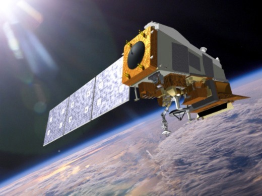
Launched in October 2011, the Suomi National Polar-orbiting Partnership (Suomi NPP) is a weather satellite aimed at demonstrating sensor capabilities, as well as provide data continuity to previous Earth Observing System (EOS) missions initiated by the National Aeronautics and Space Administration (NASA). Suomi NPP is operated by NASA and the National Oceanic and Atmospheric Administration (NOAA), with the aim of monitoring the environment on Earth and the planet’s climate.
Quick facts
Overview
| Mission type | EO |
| Agency | NASA, NOAA |
| Mission status | Operational (extended) |
| Launch date | 28 Oct 2011 |
| Measurement domain | Atmosphere, Ocean, Land, Snow & Ice |
| Measurement category | Cloud type, amount and cloud top temperature, Liquid water and precipitation rate, Atmospheric Temperature Fields, Cloud particle properties and profile, Ocean colour/biology, Aerosols, Multi-purpose imagery (ocean), Radiation budget, Multi-purpose imagery (land), Surface temperature (land), Vegetation, Albedo and reflectance, Surface temperature (ocean), Atmospheric Humidity Fields, Ozone, Trace gases (excluding ozone), Sea ice cover, edge and thickness, Soil moisture, Snow cover, edge and depth, Ocean surface winds, Atmospheric Winds |
| Measurement detailed | Cloud top height, Precipitation Profile (liquid or solid), Atmospheric pressure (over sea surface), Ocean imagery and water leaving spectral radiance, Aerosol absorption optical depth (column/profile), Ocean chlorophyll concentration, Downward long-wave irradiance at Earth surface, Cloud cover, Cloud optical depth, Precipitation intensity at the surface (liquid or solid), Aerosol optical depth (column/profile), Cloud type, Cloud imagery, Cloud base height, Aerosol Extinction / Backscatter (column/profile), Land surface imagery, Upward short-wave irradiance at TOA, Upward long-wave irradiance at TOA, Fire temperature, Vegetation type, Fire fractional cover, Earth surface albedo, Downwelling (Incoming) solar radiation at TOA, Leaf Area Index (LAI), Land cover, Atmospheric specific humidity (column/profile), O3 Mole Fraction, Atmospheric temperature (column/profile), Land surface temperature, Sea surface temperature, Sea-ice cover, Snow cover, Soil moisture at the surface, Wind speed over sea surface (horizontal), Normalized Differential Vegetation Index (NDVI), CO2 Mole Fraction, Sea-ice type, Soil type, Downward short-wave irradiance at Earth surface, Sea-ice surface temperature, Long-wave Earth surface emissivity, Atmospheric pressure (over land surface), Upwelling (Outgoing) long-wave radiation at Earth surface, Wind vector over land surface (horizontal) |
| Instruments | CERES, ATMS, CrIS, VIIRS, OMPS-L, OMPS-N |
| Instrument type | Imaging multi-spectral radiometers (vis/IR), Earth radiation budget radiometers, Atmospheric chemistry, Atmospheric temperature and humidity sounders |
| CEOS EO Handbook | See Suomi NPP (National Polar-orbiting Partnership) summary |
Summary
Mission Capabilities
Suomi NPP has five sensors onboard, they are: the Advanced Technology Microwave Sounder (ATMS), the Visible/Infrared Imager and Radiometer Suite (VIIRS), the Cross-track Infrared Sounder (CrIS), the Ozone Mapping and Profiler Suite (OMPS) and the Cloud and the Earth’s Radiant Energy System (CERES).
ATMS is a cross-track microwave radiometer that provides atmospheric temperature, moisture and pressure measurements when recorded in conjunction with CrIS, a high-resolution infrared sounder used to profile Earth’s atmosphere. VIIRS is a multispectral radiometer with a rotating telescope used to observe land, ocean and atmospheric parameters on a daily basis, and OMPS is an ultraviolet (UV) imaging spectrometer with the purpose of measuring ozone concentration variation with altitude and ozone levels in the atmosphere. Finally, CERES is used to measure reflected shortwave radiance, with measurements taken at top of atmosphere and at Earth’s surface, to continue a database of Earth-reflected solar and Earth-emitted thermal radiation.
Performance Specifications
ATMS has a swath width of 2300 km, spatial resolution of approximately 1.5 km, and 22 different measurement channels that emit at low and high frequencies to detect temperature and humidity respectively.
VIIRS also collects data in 22 spectral bands, varying between visible near infrared (VNIR) and thermal infrared (TIR) spectral ranges, with a swath width of 3000 km and a field of view (FOV) of ±55.84°. The spatial resolution is between 0.4 to 0.8 km, with the radiometric bands providing double the resolution when compared to imagery bands. CrIS has a swath width of 2300 km at a field of view of ±48.33° and a ground spatial resolution of 14 km, recorded over 1300 spectral bands across the infrared region.
OMPS utilises three spectrometers, two in the nadir sensor and one in the limb sensor. The nadir sensor images total column observations with a resolution of 0.42 nm and has a 2800 km cross-track swath using a FOV of 110°, while the nadir profile spectrometer has a 250 km cross-track swath using a FOV of 16.6°. The limb profiler uses three vertical slits to sample with a cross-track swath of 500 km, using a FOV of 8.5° and has a spectral resolution that ranges from 0.75 nm to 25 nm.
CERES utilises two identical scanners that record using three spectral channels each, with a spatial resolution of 20 km at nadir and a FOV of ±78° for cross-track.
Suomi-NPP is in a sun-synchronous near-circular polar orbit 824 km above the ground with an inclination angle of 98.74° and orbital period of 101 minutes.
Space and Hardware Components
Suomi-NPP was built by Ball Aerospace and Technologies Corporation (BATC) and utilises BATC’s Ball Commercial Platform 2000 (BCP 2000) bus. Communications with the satellite are operated using the MIL-STD-1553 data bus and can generate a real-time data stream at 15 Mbit/s.
Suomi-NPP also consists of additional ground segments that assist with satellite operation and data transfer and processing. This includes the Command Control & Communication Segment (C3S), where overall mission management and coordination of joint program operations are provided. It also provides the data network for mission data routing to ground elements and establishes communication with the NPP satellite. The Interface Data Processing Segment (IDPS) utilises raw sensor data and satellite telemetry from C3S to distribute data to the US Operational Processing Centres (OPCs).
Suomi NPP (National Polar-orbiting Partnership) Mission
Spacecraft Launch Mission Status Sensor Complement Ground Segment References
Some background on the renaming of the NPP mission
In January 2012, NASA has renamed its newest Earth-observing satellite, namely NPP (NPOESS Preparatory Project) launched on October 28, 2011, to Suomi NPP (National Polar-orbiting Partnership). This is in honor of the late Verner E. Suomi, a meteorologist at the University of Wisconsin, who is recognized widely as "the father of satellite meteorology." The announcement was made on January 24, 2012 at the annual meeting of the American Meteorological Society in New Orleans, Louisiana.
Verner Suomi (1915-1995) was born and raised in Minnesota. He spent nearly his entire career at the University of Wisconsin-Madison, where in 1965 he founded the university's Space Science and Engineering Center (SSEC) with funding from NASA. The center is known for Earth-observing satellite research and development. In 1964, Suomi served as chief scientist of the U.S. Weather Bureau for one year. Suomi's research and inventions have radically improved weather forecasting and our understanding of global weather.
NPP is a joint NASA/IPO (Integrated Program Office)/NOAA LEO weather satellite mission initiated in 1998. The primary mission objectives are:
1) To demonstrate the performance of four advanced sensors (risk reduction mission for key parts of the NPOESS mission) and their associated Environmental Data Records (EDR), such as sea surface temperature retrieval.
2) To provide data continuity for key data series observations initiated by NASA's EOS series missions (Terra, Aqua and Aura) - and prior to the launch of the first NPOESS series spacecraft. Because of this second role, NPP is sometimes referred to as the EOS-NPOESS bridging mission.
Three of the mission instruments on NPP are VIIRS (Visible/Infrared Imager and Radiometer Suite), CrIS (Cross-Track Infrared Sounder), and OMPS (Ozone Mapping and Profiler Suite). These are under development by the IPO. NASA/GSFC developed a fourth sensor, namely ATMS (Advanced Technology Microwave Sounder). This suite of sensors is able to provide cloud, land and ocean imagery, covering the spectral range from the visible to the thermal infrared, as well as temperature and humidity profiles of the atmosphere, including ozone distributions. In addition, NASA is developing the NPP S/C and providing the launch vehicle (Delta-2 class). IPO is providing satellite operations and data processing for the operational community; NASA is supplying additional ground processing to support the needs of the Earth science community. 3) 4) 5) 6) 7) 8)
CERES instrument selected for NPP and NPOESS-C1 missions: 9)
In early 2008, the tri-agency (DOC, DoD, and NASA) decision gave the approval to add the CERES (Clouds and the Earth's Radiant Energy System) instrument of NASA/LaRC to the NPP payload. The overall objective of CERES is to provide continuity of the top-of-the-atmosphere radiant energy measurements - involving in particular the role of clouds in Earth's energy budget. Clouds play a significant, but still not completely understood, role in the Earth's radiation budget. Low, thick clouds can reflect the sun's energy back into space before solar radiation reaches the surface, while high clouds trap the radiation emitted by the Earth from escaping into space. The total effect of high and low clouds determines the amount of greenhouse warming. - CERES products include both solar-reflected and Earth-emitted radiation from the top of the atmosphere to the Earth's surface.
In addition, the tri-agency decision called also for adding two instruments, namely CERES and TSIS (Total Solar Irradiance Sensor), to the payload of the NPOESS-C1 mission.
Background: The CERES instrument is of ERBE (Earth Radiation Budget Experiment) heritage of NASA/LaRC, first flown on the ERBS (Earth Radiation Budget Satellite) mission, launch Oct. 5, 1984, then on NOAA-9 (launch Dec. 12, 1984), and NOAA-10 (launch Sept. 17, 1986). The CERES instrument is flown on TRMM (Tropical Rainfall Measuring Mission), launch Nov. 27, 1997, as a single cross-track radiance sensor of short (0.3-5 μm), long- (8-12 μm) and total wave (0.3-100 μm; prototype flight model flown on TRMM). Two further advanced CERES instrument assemblies are also being flown on NASA's Terra mission (launch Dec. 18, 1999) as a dual-track scanner (two radiometers) in XT (Cross-Track ) support or in a RAPS (Rotational Azimuth Plane Scan) support mode. Another CERES instrument system (two radiometers) are being flown on Aqua of NASA (launch May 4, 2002).
The CERES instrument on NPP will provide continuity the long climate data record of the Earth's radiant energy.
JPSS (Joint Polar Satellite System) - NPOESS program terminated 10
In Feb. 2010, the NPOESS (National Polar-orbiting Environmental Satellite System) tri-agency program was terminated by the US government due to severe cost overruns and program delays. In 2009, an IRT (Independent Review Team) concluded that the current NPOESS program, in the absence of managerial and funding adjustments, has a low probability of success and data continuity is at extreme risk. The Office of Science and Technology, with the Office of Management and Budget and the National Security Council, as well as representatives from each agency, examined various options to increase the probability of success and reduce the risk to data continuity.
NOAA's restructured satellite program, the civilian JPSS (Joint Polar Satellite System), was created in the aftermath of the White House's Feb. 2010 decision to cancel NPOESS. The development of the new JPSS will be managed by NASA/GSFC while the spacecraft will be owned and operated by NOAA. The launch of JPSS-1 is planned for 2017.
NOAA, through NASA as its acquisition agent, will procure the afternoon orbit assets that support its civil weather and climate requirements and DoD will independently procure assets for the morning orbit military mission - referred to as DWSS (Defense Weather Satellite System). Both agencies will continue to share environmental measurements made by the system and support the operations of a shared common ground system.
The Administration decision for the restructured Joint Polar Satellite System will continue the development of critical Earth observing instruments required for improving weather forecasts, climate monitoring, and warning lead times of severe storms. NASA’s role in the restructured program will be modeled after the procurement structure of the successful POES (Polar Operational Environmental Satellite) and GOES (Geostationary Operational Environmental Satellite) programs, where NASA and NOAA have a long and effective partnership. The partner agencies are committed to maintaining collaborations towards the goal of continuity of earth observations from space.
The restructured Joint Polar Satellite System is planned to provide launch readiness capability in FY 2015 and FY 2018 (with launches of JPSS-1 in 2016 and JPSS-2 in 2019, respectively) in order to minimize any potential loss of continuity of data for the afternoon orbit in the event of an on orbit or launch failure of other components in the system. Final readiness dates will not be baselined until all transition activities are completed.
The NPP project, as preparatory mission for the NPOESS program, received its OK to continue in the early spring of 2010. However, the close partnership with NPOESS can still be seen in all the references throughout the documentation of this file.
NPP serves as a bridge mission between NASA's EOS (Earth Observing System) series of satellites and the next-generation JPSS (Joint Polar Satellite System), a NOAA program that will also collect weather and climate data.
NPP will provide on-orbit testing and validation of sensors, algorithms, ground-based operations, and data processing systems that will be used in the operational JPSS mission. By 2016, the first JPSS spacecraft will be launched into the afternoon orbit to provide significantly improved operational capabilities and benefits to satisfy critical civil and national security requirements for spaceborne, remotely sensed environmental data. The last satellite in the JPSS mission constellation is expected to continue operations until about 2037.
Spacecraft
The Suomi NPP spacecraft has been built and integrated by BATC (Ball Aerospace and Technologies Corporation) of Boulder, CO (NASA/GSFC contract award in May 2002). The platform design is a variation of BATC's BCP 2000 (Ball Commercial Platform) bus of ICESat and CloudSat heritage. The spacecraft consists of an aluminum honeycomb structure. 12) 13) 14)
The ADCS (Attitude Determination and Control Subsystem) provides 3-axis stabilization using 4 reaction wheels for fine attitude control, 3 torquer bars for momentum unloading, thrusters for coarse attitude control (such as during large-angle slews for orbital maintenance), 2 star trackers for fine attitude determination, 3 gyros for attitude and attitude rate determination between star tracker updates, 2 Earth sensors for safe-mode attitude control, and coarse sun sensors for initial attitude acquisition, all monitored and controlled by the spacecraft controls computer. ADCS provides real-time attitude knowledge of 10 arcsec (1 sigma) at the S/C navigation reference base, real-time spacecraft position knowledge of 25 m (1 sigma), and attitude control of 36 arcsec (1 sigma).
The EPS (Electrical Power Subsystem) uses GaAs solar cells to generate an average power of about 2 kW (EOL). The solar array rotates once per orbit to maintain a nominally normal orientation to the sun). In addition, a single-wing solar array is mounted on the anti-solar side of the S/C; its function is to preclude thermal input into the sensitive cryo radiators of the VIIRS and CrIS instruments. A regulated 28 ±6 VDC power bus distributes energy to all S/C subsystems and instruments. A NiH (Nickel Hydrogen) battery system provides power for eclipse phase operations.
The C&DHS (Command & Data Handling Subsystem) collects instrument data (12 Mbit/s max total) via an IEEE 1394a-2000 “FireWire” interface (VIIRS, CrIS and OMPS instruments), and stores the data on board. Communications with ATMS occurs across the MIL-STD-1553 data bus. A new 1394/FireWire chipset was developed for the communication support, bringing spaceborne communications (onboard data handling and RF data transmission) onto a new level of service range and performance.
Upon ground command or autonomously, the C&DHS transmits stored instrument data to the communication system for transmission to the ground. Also, the C&DHS generates a real-time 15 Mbit/s data stream consisting of instrument science and telemetry data for direct broadcast via X-band to in-situ ground stations.
Parameter | Value | Parameter | Value |
S/C dimensions | 1.3 m x 1.3 m x 4.2 m | S/C total mass | ~2200 kg |
Instrument data rate | 12.5 Mbit/s | Payload mass | 464 kg |
Downlink data rate | 300 Mbit/s in X-band | Position knowledge | 75 m each axis |
The spacecraft is designed to be highly autonomous. For satellite safety, the S/C controls computer monitors spacecraft subsystem and instrument health. It can take action to protect itself (for example, in the event of an anomaly that threatens the thermal or optical safety and health of the S/C, then it can enter into a safe or survival mode and stay in the mode indefinitely until ground analysis and resolution of the anomaly). In addition, the satellite is designed to require infrequent uploads of commands (the instruments operate mainly in a mapping mode and therefore require few commands even for periodic calibration activities, and a sufficiently large command buffer is available for storage of approximately 16 days of commands).
The spacecraft has an on-orbit design lifetime of 5 years (available consumables for 7 years). The S/C dry mass is about 1400 kg. NPP is designed to support controlled reentry at the end of its mission life (via propulsive maneuvers to lower the orbit perigee to approximately 50 km and target any surviving debris for open ocean entry). NPP is expected to have sufficient debris that survives reentry so as to require controlled reentry to place the debris in a pre-determined location in the ocean.
Launch
Launch: The NPP spacecraft was launched on October 28, 2011 on a Delta-2-7920-10 vehicle from VAFB, CA (launch provider: ULA). The launch delay of nearly a year was due to development/testing problems of the CrIS (Cross-track Infrared Sounder) instrument. 15) 16) 17)
Orbit: Sun-synchronous near-circular polar orbit (of the primary NPP), altitude = 824 km, inclination =98.74º, period = 101 minutes, LTDN (Local Time on Descending Node) at 10:30 hours. The repeat cycle is 16 days (quasi 8-day).
Secondary payloads: The secondary payloads on the Suomi NPP mission are part of NASA's ElaNa-3 (Educational Launch of Nanosatellites) initiative. All secondary payloads will be deployed from standard P-PODs (Poly Picosatellite Orbital Deployer). 18)
• AubieSat-1, a 1 U CubeSat of AUSSP (Auburn University Student Space Program), Auburn, AL, USA.
• DICE (Dynamic Ionosphere CubeSat Experiment), two nanosatellites (1.5U CubeSats) of the DICE consortium (Utah State University, Logan, UT, USA) with a total mass of 4 kg.
• E1P-2 (Explorer-1 PRIME-2) flight unit-2, a CubeSat mission of MSU (Montana State University), Bozeman, MT, USA.
• RAX-2 (Radio Aurora eXplorer-2), an NSF-sponsored 3U CubeSat of the University of Michigan, Ann Arbor, MI, USA
• M-Cubed (Michigan Multipurpose Minisat), a 1U CubeSat of the University of Michigan, Ann Arbor, MI. M-Cubed features also the collaborative JPL payload called COVE (CubeSat On-board processing Validation Experiment).
Orbit of the secondary payloads: After the deployment of the NPP primary mission, the launch vehicle transfers all secondary payloads into an elliptical orbit for subsequent deployment. This is to meet the CubeSat standard of a 25 year de-orbit lifetime as well as the science requirements of the payloads riding on this rocket. The rocket will take care of the maneuvering and when it reaches the correct orbit, it will deploy all of the secondary payloads, into an orbit of ~ 830 km x ~ 350 km, inclination = 99º.
RF Communications
The NPP satellite collects instrument data, stores the data onto a solid-state recorder of about 280 Gbit capacity. A two-axis gimbaled X-band antenna is mounted on a post above the payload to provide a high bandwidth downlink. Source science data are generated at a rate of about 12.5 Mbit/s. Global, or stored mission data will be downlinked at X-band frequencies (8212.5 MHz, data rate of 300 Mbit/s) to a 13 m ground receiving station located at Svalbard, Norway.
Two wideband transmissions carry NPP mission data: SMD (Stored Mission Data) and HRD (High-Rate Data). These transmissions are distinct from the narrowband data streams containing the satellite's housekeeping telemetry. Mission data are collected from each of the five instruments (ATMS, VIIRS, CrIS, OMPS, CERES).
These data, along with spacecraft housekeeping data, are merged and provided to the ground on a real-time 15 Mbit/s downlink, called HRD direct broadcast. Instrument and housekeeping data are also provided to the SSR (Solid State Recorder) for onboard storage and playback as SMD. The SMD are stored in the spacecraft's SSR and downlinked at 300 Mbit/ss through playback of the SSR once per orbit over the NPP/NPOESS SvalSat ground station in Svalbard, Norway.
The HRD stream is similar to the SMD as it consists of instrument science, calibration and engineering data, but it does not contain data from instrument diagnostic activities. The HRD is constantly transmitted in real time by the spacecraft to distributed direct broadcast users. Output to the HRD transmitter is at a constant 15 Mbit/s rate.
Data acquisition: In early 2004, IPO in cooperation with NSC (Norwegian Space Center), installed a 13 m antenna dish - a dual X/S-band configuration, at SGS (Svalbard Ground Station), located at 78.216º N, 20º E on the Norwegian Svalbard archipelago (also referred to as Spitzbergen) near the town of Longyearbyen. The SGS complex is owned by the Norwegian Space Center (Norsk Romsenter), Oslo, Norway, and operated by the Tromsø Satellite Station (TSS) through its contractor KSAT (Kongsberg Satellite Services). SGS is the primary data downlink site for global stored mission data (SMD) from NPP. Svalbard is located at a high enough latitude to be able to “see” (i.e., track) all 14 daily NPP satellite passes. 19)
The global NPP data will be transmitted from Svalbard within minutes to the USA via a fiber-optic cable system that was completed in January 2004 as a joint venture between the IPO, NASA, and NSC. Once the data stream is in the USA, the RDRs (Raw Data Records) will be processed into SDRs (Sensor Data Records) and EDRs by the Interface Data Processing Segment (IDPS). The performance goal calls for EDR delivery within 3 hours of acquisition. - NPP also focuses on ground segment risk reduction by providing and testing a subset of an NPOESS-like ground segment. Developed algorithms can be thoroughly tested and evaluated. This applies also to the methods of instrument verification, calibration, and validation.
Note: The new antenna and fiber-optic link at SGS are already being used to acquire data of five to ten Coriolis/WindSat passes/day and delivery of the data to users in a reliable and timely manner. Subsequent to the NPP mission, the Svalbard site and the high-speed fiber-optic link will also serve as one node in a distributed ground data communications system for NPOESS acquisition service.
The TT&C function uses S-band communications with uplink data rates of up to 32 kbit/s and downlink rates of up to 128 kbit/s. The NOAA network of polar ground stations will be used for mission operations (back-up TT&C services via TDRSS through S-band omni antennas on the satellite).
Suomi NPP broadcast services
In addition, NPP will have a real-time HRD (High Rate Data) downlink in X-band (7812.0 MHz ± 0.03 MHz) direct broadcast mode to users equipped with appropriate field terminals. The objectives are to validate the innovative operations concepts and data processing schemes for NPOESS services. NPP world-wide users will already experience NPOESS-like data well in advance of the first NPOESS flight in 2013. The NPP broadcast services to the global user community are: 21) 22) 23) 24)
• X-band downlink at 30 Mbit/s
• Convolutional coding
• QPSK (Quadra-Phase Shift Keying) modulation
• An X-band acquisition system of 2.4 m diameter aperture is sufficient for all data reception. NASA will provide:
• Real-Time Software Telemetry Processing System
• Ground-Based Attitude Determination module
• Stand-alone Instrument Level-1 and select Level-2 (EDR) algorithms
• Instrument-specific Level 1 (SDR) & select Level-2 (EDR) visualization & data formatting tools
The DRL (Direct Readout Laboratory) of NASA/GSFC is committed to promote continuity and compatibility among evolving EOS direct broadcast satellite downlink configurations and direct readout acquisition and processing systems. The DRL bridges the EOS missions with the global direct readout community by establishing a clear path and foundation for the continued use of NASA’s Earth science DB data. The DRL is also involved in continued efforts to ensure smooth transitions of the Direct Broadcast infrastructure from the EOS mission to the next generation NPP (NPOESS Preparatory Project) and NPOESS (National Polar-orbiting Operational Environmental Satellite System) missions in the future. In an effort to foster global data exchange and to promote scientific collaboration, the DRL with support from other groups, is providing the user community access to Earth remote sensing data technologies and tools that enable the DB community to receive, process, and analyze direct readout data.
DRL developed IPOPP (International Polar Orbiter Processing Package), the primary processing package that will enable the Direct Readout community to process, visualize, and evaluate NPP and NPOESS sensor and EDRs (Environmental Data Records), which is a necessity for the Direct Readout community during the transition from the Earth Observing System (EOS) era to the NPOESS era. DRL developed also the NISGS (NPP In-Situ Ground System). The IPOPP will be: 25)
• Freely available
• Portable to Linux x86 platforms
• Efficient to run on modest hardware
• Simple to install and easy to use
• Able to ingest and process Direct Broadcast overpasses of arbitrary size
• Able to produce core and regional value-added EDR products.
Parameter | High Data Rate | Low Data Rate |
Carrier frequency: | 7812 MHz NPP |
|
Max occupied bandwidth: NPP | 30 MHz NPP |
|
Channel data rate: (includes all CCSDS overhead, Reed-Solomon forward error correction, and convolutional encoding) | 30 Mbit/s NPP |
|
Ground antenna aperture size | 2-3 m | 1 m |
Minimum elevation angle | 5º | 5º |
VIIRS compression | Lossless – RICE | Lossy – JPEG2000 |
Note: As of May 2021, the previously large SuomiNPP file has been split into three files, to make the file handling manageable for all parties concerned, in particular for the user community.
• This article covers the SuomiNPP mission and its imagery in the period 2021
• SuomiNPP imagery in the period 2020-2019
• SuomiNPP imagery in the period 2018-2011
Mission Status
• July 25, 2022: Though much of the far southern hemisphere is bathed in winter darkness, there was a bit of light last week. The aurora australis, or southern lights, fluttered north and south of the Antarctic Circle on several nights. 26)
- In the image, the sensor was actually detecting the light emissions as energetic particles rained down from Earth’s magnetosphere into the upper atmosphere. Fast-moving electrons from space collide with oxygen and nitrogen molecules in the ionosphere and chemically excite them. As the gases return to their normal state, they emit small bursts of energy in the form of light (photons); oxygen molecules and atoms tend to glow green, white, or red, while nitrogen tends to be blue or purple. This ghostly light originates at altitudes of 100 to 400 km (60 to 250 miles).
- Solar Cycle 25 is now underway and more sunspots and solar storms are starting to emerge, which should bring more opportunities to see auroras in both hemispheres. Solar cycles are traditionally measured by the rise and fall in the number of sunspots, but they also coincide with increases in solar flares, coronal mass ejections (CMEs), radio emissions, and other forms of space weather. Scientists have forecasted that the Sun should reach its next peak of activity (solar maximum) in mid-2025.
• July 15, 2022: In June and July 2022, heatwaves struck Europe, North Africa, the Middle East, and Asia, as temperatures climbed above 40 degrees Celsius (104 degrees Fahrenheit) in places and broke many long-standing records. 27)
- In Western Europe, which was already experiencing severe drought, the heatwave fueled fires that raged across Portugal, Spain, and parts of France. In Portugal, temperatures reached 45 degrees Celsius (113 degrees Fahrenheit) on July 13 in the town of Leiria, where more than 3,000 hectares (7,400 acres) had burned. More than half of the country was on red alert as firefighters battled 14 active fires.
- In Italy, the record heat contributed to the July 3 collapse of a portion of the Marmolada Glacier in the Dolomites. The avalanche of snow, ice, and rock killed 11 hikers.
- In the U.K., the Met Office issued extreme heat or amber warnings as temperatures were expected to continue to climb, possibly breaking all-time highs.
- In North Africa, Tunisia has endured a heatwave and fires that have damaged the country's grain crop. On July 13 in the capital city of Tunis, the temperature reached 48 degrees Celsius (118 degrees Fahrenheit), breaking a 40-year record.
- In Iran, temperatures remained high in July after reaching a scorching 52 degrees Celsius (126 degrees Fahrenheit) in late June.
- In China, the summer has brought three heatwaves that have buckled roads, melted tar, and popped off roof tiles. The Shanghai Xujiahui Observatory, where records have been kept since 1873, recorded its highest temperature ever: 40.9 degrees Celsius (105 degrees Fahrenheit) on July 13, 2022. High humidity and dewpoints, along with warm overnight temperatures, created potentially deadly conditions.
• July 6, 2022: Alaskan summers have long been described as brief and mild. In the early summer of 2022, the word that stood out was smoky. 28)
- Smoke from one particularly smoky fire northwest of Iliamna Lake (southwest Alaska) hampered visibility on the Seward Peninsula, more than 400 miles (600 kilometers) to the northwest. The influx of smoke led to extremely high particulate matter readings (AQI above 700 at times) in Nome, according to University of Alaska Fairbanks climatologist Rick Thoman.
- Alaska surpassed 2 million acres (8000 km2) burned on July 2, 2022, matching the earliest date for the milestone in the past 20 years. On July 5, 2022, the Alaska Interagency Coordination Center reported 210 active fires in the state. Forty-two were large fires with firefighters working on them, according to the National Interagency Fire Center. Wildfires are a regular feature of Alaskan summers, but this year’s fires have been exacerbated by drought, unusual heat, and several intense lightning storms. In early July, the area burned was on track to be among the largest on record, according to Thoman.
• March 2, 2022: Ecologists and biologists have long recognized that artificial light at night can have adverse effects on the health of humans and terrestrial wildlife, including disrupted sleep patterns, feeding schedules, and reproductive cycles. 30)
- A growing body of research is showing that marine life is also sensitive to artificial light, including extremely low levels and certain wavelengths, particularly blue and green light. Now, for the first time, scientists have quantified underwater light levels for coastal zones around the world. A team of researchers from England, Norway, and Israel have released the first global atlas of artificial light in the sea. 31)
- “These very low light levels that artificial light generates are critically important for biological organisms,” said lead author and oceanographer Tim Smyth, who specializes in marine optics and remote sensing of ocean color at Plymouth Marine Laboratory. “But how much of an impact it has in the marine environment has been pretty understudied.”
- The study gives researchers a guide to where they should focus future studies of the effects of artificial light on marine life. In particular, Smyth said, the study highlights areas where ecosystems are particularly stressed by artificial light, which could lead to rapid evolutionary changes and adaptation.
- “The effects of artificial light in marine ecosystems should be a real focus for global change research,” Smyth said.
- The scientists found that 1.9 million km2 (735,000 square miles) of the ocean experience biologically significant amounts of artificial light pollution to a depth of 1 meter (3 feet). This represents about 3 percent of the world’s Exclusive Economic Zones (EEZs)—the area extending 370 kilometers (200 nautical miles) off a country’s coast. Significant areas of the ocean are seeing light exposures to depths of 10 meters (33 feet), 20 meters (66 feet), or more.
- The depth to which light can penetrate depends not only on the intensity of light above water, Smyth said, but also on the optical properties of the water, which vary seasonally. For example, in areas with very clear water, including part of the South China Sea near Malaysia, light at night can reach depths of more than 40 meters.
- Some of the most extensive marine light pollution occurs in areas where offshore oil and gas platforms, wind farms, and island development brighten the night above and below the water line. The maps above show the North Sea in April and the Persian Gulf in December. They include both sky brightness above water and the critical depth to which underwater light is reaching. (Note the different scales for each.)
- Artificial light is very different from natural light in its spectral properties, intensity, and timing, Smyth said. Artificial lights switch on abruptly at dusk and burn throughout the night, every night, whereas natural nighttime light, like moonlight, waxes and wanes on daily, monthly, and seasonal timescales.
- Many marine species have evolved biological functions that are governed by natural light cycles, even at low levels and at great depths, and some are attuned to certain wavelengths of light. For example, copepods are particularly sensitive to moonlight, which signals their daily migration up and down the water column to feed. Copepods are keystone organisms in many marine food webs. For the study, the researchers used the light sensitivity of copepods as the threshold for a biologically significant amount of light.
- A foundational piece of the new research was a global atlas of artificial night sky brightness published by Fabio Falchi, a physicist at the Light Pollution Science and Technology Institute (Italy) and colleagues in 2016. That atlas was built on data from the Visible Infrared Imaging Radiometer Suite (VIIRS) on the Suomi National Polar-orbiting Partnership (NPP) satellite, which can observe dim lights with its day-night band (DNB).
- “We used ocean-color satellite products to construct climatologies for every month of the year, everywhere in the global ocean,” Smyth said. The model could then calculate how the above-water light—now split into its red, green, and blue components—would propagate underwater based on the optical properties of water at a given location in a given month.
- Coastal zones are home to many of the largest urban areas on Earth. As they continue to grow, skyglow—the scattering and diffusion of light by clouds, fog, and pollutants in the atmosphere—seeping into the sea, may grow as well, Smyth said.
- Additionally, efforts by urban planners to transition to more energy-efficient light-emitting diode (LED) lighting could also adversely affect marine ecosystems, he said. Cities that once glowed orange under sodium vapor lights now give off a harsher blue glow and a broader spectrum of light that could affect marine species.
• February 8, 2022: Auroras are a brilliant reminder that Earth is constantly absorbing energy from the Sun—even on the night side. Our nearest star bathes the planet in streams of energetic particles, magnetic fields, and radiation that stimulate our atmosphere and occasionally light up the night sky. 32)
- The auroras were a visible manifestation of a minor geomagnetic storm—a disturbance of the upper atmosphere caused by the interaction of pressure waves and electromagnetic energy from the Sun interacting with Earth’s magnetic field (or magnetosphere). In this case, the Sun was spewing streams of high-speed solar wind through a temporary hole in the solar corona.
- The collision of solar particles and pressure into Earth’s magnetosphere accelerates particles already trapped in the space around Earth (such as in the radiation belts). Those particles are sent crashing into Earth’s upper atmosphere at altitudes of 100 to 400 km (60 to 250 miles), where they excite oxygen and nitrogen molecules and release photons. The results are rays, sheets, and curtains of dancing light in the sky.
- Solar Cycle 25 is now underway, and that means more frequent opportunities to see auroras. Solar cycles are traditionally measured by the rise and fall in the number of sunspots, but they also coincide with increases in solar flares, coronal mass ejections (CMEs), radio emissions, and other forms of space weather. Scientists have forecasted that the Sun will reach its next peak of activity (solar maximum) in mid-2025.
- You can participate in aurora citizen science through a project called Aurorasaurus. The project tracks auroras around the world via reports to its website and on Twitter, then generates a real-time global map of those reports. Citizen scientists verify the tweets and reports, and each verified sighting serves as a valuable data point for scientists to analyze and incorporate into space weather models. The project is a public-private partnership with the New Mexico Consortium and supported by the National Science Foundation and NASA.
• January 26, 2022: In late January 2022, a substantial dust storm enveloped the Arabian Sea. Plumes of desert dust affected populated areas around the basin, as winds carried the particles over Karachi, Mumbai, and numerous other cities and degraded air quality. 33)
- Dust arose from three different countries but merged into a large plume that cast a pall over much of the Arabian Sea. According to Hiren Jethva, a Morgan State University scientist based at NASA’s Goddard Space Flight Center, the size of the plume was “quite remarkable,” as was its unusual path.
- Initially on January 21, high winds associated with a low-pressure system whipped up dust and carried it toward the southeast. On January 22, the dust blew over the sea and then hooked toward the east. By January 23, dust blanketed western India, shrouding the states of Maharashtra, Gujarat, and Rajasthan.
- According to Jethva, winter winds usually blow out from India toward the Arabian Sea, carrying various aerosols from local pollution and biomass burning. “However, the reversal of wind direction has likely occurred, bringing dust from the ocean to the Indian subcontinent,” Jethva said.
- The dust hung in the air for days. In Mumbai, the air quality index on January 24 was “severe,” the highest of six categories in the country’s index. According to news reports, an air quality index that high in Mumbai is “unprecedented.” Toward the southeast, the city of Pune saw air quality in the “very poor” category, ranking worse that day than Delhi, where winter air quality is often affected by temperature inversions.
- The dust storm was accompanied by chilly weather. According to news reports, the dust in Mumbai contributed to the lowest daytime January temperature recorded in the city in a decade, reaching just 23.8°C (74.8°F) on January 23. On average, daytime temperatures in January reach 31°C (88°F).
• January 8, 2022: The glow of a volcanic eruption in the Galápagos Islands was captured by the Visible Infrared Imaging Radiometer Suite (VIIRS) on the NOAA-NASA Suomi NPP satellite. The image, acquired by the VIIRS “day-night band” at 1:20 a.m. local time (7:20 UTC) on January 7, 2022, shows lava spewing from Wolf Volcano, on the northern end of Isabela Island. The largest island in the Galápagos archipelago lies roughly 1,100 km (700 miles) off the west coast of Ecuador. 34)
- According to the Geophysical Institute in Quito, the volcano began erupting late on January 6, sending incandescent lava flows down the volcano’s flanks and ejecting ash clouds up to about 3,800 meters (12,500 feet). Later on January 7, the Moderate Resolution Imaging Spectroradiometer (MODIS) on NASA’s Terra satellite acquired an image of the plume blowing west over the Pacific Ocean.
- Wolf is the largest and tallest volcano in the Galápagos Islands. It last erupted in May and June 2015, with an eruption rated 4 on the Volcanic Explosivity Index (VEI) (range from 0 to 8). One of the volcano’s earlier eruptions, in 1797, was the first historical eruption documented in the Galápagos Islands.
- Isabela Island is home to the critically endangered pink land iguana. The isolation of the islands and their location at the confluence of major ocean currents gave rise to unique species, including the land iguana, the giant tortoise, and many varieties of finch. The Galápagos archipelago is a UNESCO World Heritage site.
• December 29, 2021: The arrangement of lines in this image might look like an oceanic game of tic-tac-toe, but in fact, the grid can be explained by a relatively common atmospheric feature. Ship tracks are long, narrow clouds that form in the sky over the ocean when water vapor condenses around tiny particles in ship exhaust. 35)
- Trails of aerosol pollution from ships are present with or without the clouds. But the presence of these numerous tiny particles can become more apparent in natural-color images when the particles interact with low-level clouds and cause them to brighten. This happens because aerosols allow more and smaller cloud droplets to form, providing more surfaces to reflect light.
- Scientists have been studying the phenomenon for decades, teasing out the complex interactions between aerosols and clouds to decipher what those interactions mean for climate change. For instance, scientists want to know the extent that ship tracks can lead to cooling across the planet.
- In recent years, scientists have been using machine learning to help identify ship tracks—some of which can go undetected by human eyes—and to classify various cloud types around the planet. The technique is helping to grow the collection of cloud images available for scientific study.
• December 18, 2021: Typhoon Rai crossed the southern and central Philippines on December 16, 2021, having intensified to category 5 strength just hours before landfall. Locally named Odette, the storm was one of the strongest recorded on Earth this year and the sixth to reach category 5. 36)
- News and weather reports indicated that the storm first came ashore in Siargao, a popular island for tourism, with sustained winds around 195 kilometers (120 miles) per hour, before crossing over several other islands. About 100,000 people evacuated their homes before Rai arrived. An estimated 30 million people live in the central and southern islands of the Philippines.
- Forecasters from the U.S. Joint Typhoon Warning Center predicted that the storm would head toward Vietnam and southern China in the coming days.
- Rai (Odette) is the 15th typhoon to pass through or close to the Philippines this year. The archipelago typically sees more landfalling storms annually than any other place on Earth.
• December 14, 2021: On the night of December 10, 2021, a potent storm front brought tornadoes, intense thunderstorms, and bursts of straight-line wind to the Midwestern United States. Though tornadoes can occur in any time of year—with roughly a dozen every December—the event was rare for how long it lasted and how far north it occurred in meteorological winter. 37)
- With unseasonably warm and humid weather in place in the mid-section of the U.S. and a cool weather front approaching from the west, the National Weather Service (NWS) predicted early on December 10 that severe weather was imminent: “A few strong tornadoes, damaging gusts, and large hail are all expected beginning this evening across Arkansas and Missouri, with the greatest tornado threat close to the confluence of the Mississippi and Ohio Rivers.”
- A few hours later, as many as 70 tornado-like events were reported across the Midwest, killing at least 100 people and injuring hundreds more in Arkansas, Kentucky, Illinois, and Missouri. Preliminary reports suggest it was the deadliest tornado event in the U.S. since a tornado hit Joplin, Missouri, in 2011.
- The worst damage came along what may be a historically long track for a tornadic storm that started in Arkansas and crossed through Missouri, Tennessee, and Kentucky for several hours. NWS reported winds ranging from 158 to 206 miles (254 to 332 kilometers) per hour, damage of at least an EF-3 rating on the Enhanced Fujita (EF) scale, and a ground track that may have blown across 200 miles (300 kilometers) and spanned 0.75 miles (1.2 kilometers) at its widest.
- According to meteorologist Bob Henson: “No U.S. tornado is known to have killed more than 80 people outside the core tornado season from March to June.” He added that until last weekend, the death toll for tornadoes in the U.S. in 2021 had been only 14, the third lowest since 1875.
- Several researchers reported on social media that plumes from some of the supercell thunderstorms may breached the lower edge of the stratosphere. A NASA team has been working with satellite imagery—particularly GOES weather satellites—to find signatures of tornadoes and extreme thunderstorms in such lofty plumes.
- In the most recent report from the Intergovernmental Panel on Climate Change (IPCC), scientists drew an unequivocal link between human activity and global warming. The authors of that report noted that tropical cyclones, severe storms, and dust storms are expected to become more extreme in North and Central America as the world continues to warm.
• November 2, 2021: Like a sea captain tracking a white whale, Steve Miller has been chasing “milky seas” for decades. He has been looking for examples of a rare form of marine bioluminescence, and the arrival of new night-light sensing satellite instruments has allowed him to detect several of these rare events. It also has given scientists a better chance to sample future events. 38)
- Milky seas are a rare form of bioluminescence that mariners have described as looking like a snow field spread across the ocean. The steady white glow can stretch for vast distances, and it is not disturbed by ship wakes. Sailors have sporadically encountered this phenomenon since at least the 1600s, and Jules Verne dropped a reference to it into Twenty Thousand Leagues Under the Sea.
- “A cool thing about milky seas is that they are so elusive, usually out on the high seas and away from major shipping lanes,” Miller noted. “As a result, they have remained mostly a part of maritime folklore.”
- Though there has been just one direct sampling of the phenomenon, scientists believe it occurs when populations of luminous (light-making) bacteria such as Vibrio harveyi explode in connection with colonies of certain algae and phytoplankton. Unlike typical bioluminescence—where phytoplankton emit light when they are stimulated, flashing briefly like fireflies—the bacteria in milky seas can stay lit for days to weeks. However, very little is known about the conditions in which they thrive.
- In the early 2000s, while working for the U.S. Naval Research Laboratory, Miller and colleagues began discussing the unique light signals that they might be able to detect with the Visible Infrared Imaging Radiometer Suite (VIIRS) that was being developed for the next generation of NOAA and NASA satellites. In particular, they were thinking about whether VIIRS would be able to detect any previously undetectable phenomena from space, such as bioluminescence in the ocean.
- Miller then happened upon a ship captain’s report of a strange case of glowing seas off of Somalia in 1995. That story of the S.S. Lima led Miller to look at nighttime data from the Operational Linescan System of the U.S. Defense Meteorological Satellite Program. The signal was faint and the data were very noisy, but he found that what the Lima captain reported from the sea surface was actually visible from space. Miller and colleagues published those findings in 2005 and then waited patiently for the 2011 launch of the Suomi NPP satellite, the first to carry the new VIIRS instrument.
- VIIRS was developed with a “day-night band” (DNB), a special sensor designed to detect light in a range of wavelengths from green to near-infrared. The DNB is sensitive to light levels up to 10 million times fainter than daylight, enabling scientists to distinguish signals such as airglow, auroras, city lights, and reflected moonlight. When he joined the Cooperative Institute for Research in the Atmosphere at Colorado State University in 2007, Miller continued to build a team to calibrate and explore the new features of the DNB. He believed it could help him find the elusive milky seas.
- On one track, Miller built upon an established list of milky sea sightings compiled by marine biologist Peter Herring. Miller compiled more than 200 mentions of glowing seas found in historical documents and ship reports. He found one unlikely report from the captain of the C.S.S. Alabama in 1864 off the coast of Somalia that bore uncanny similarity to the 1995 Lima event. Mapping those reports from the past two centuries, Miller and colleagues found that the majority came from the northwest Indian Ocean and Arabian Sea, as well as the waters near Indonesia and the Maritime Continent.
- On another track, Miller faced many challenges in determining whether the faint, ephemeral signal of milky seas could be detected by VIIRS. The day-night band is sensitive enough to detect many forms of nighttime light on and over the ocean—including lights from boats and gas flares from drilling platforms—and even in the sky—including airglow and atmospheric gravity waves. Clouds and snow also reflect light at night, muddying the DNB signals. Then there is the Moon: For half of every month, moonlight is the dominant signal reflecting off the ocean surface, making it hard to see much else.
- All of these signals tend to be brighter and more ubiquitous than milky seas, so all they had to be ruled out before Miller could say whether light was coming from the ocean itself. He also noted that the DNB response to light emissions is a bit “red-shifted” away from the presumed blue/green light emissions of most forms of marine bioluminescence.
- In new research published in July 2021, Miller and eight colleagues demonstrated that VIIRS could indeed detect the ghostly luminescence. Reviewing VIIRS data from 2012-2021, they found 12 instances of milky seas across the Indian Ocean and far Western Pacific (Figure 32). The signals from each event were invisible during the day—and so not attributable to some other reflective substance in the ocean—and persistent across several consecutive nights, drifting with the surface currents. 39)
- To date, the only in situ study of milky seas occurred in 1985—a chance encounter by a scientific research vessel near Socotra in the Arabian Sea. Miller would like to change that. Since the Suomi NPP and NOAA-20 satellites are both equipped with VIIRS day-night bands and make daily observations, it is possible that scientists could detect a milky sea event from space and then send a research ship out to sample the waters.
- “The reports over the years have been more or less consistent, but there remains a great deal of uncertainty in terms of what circumstances conspire to form one, as well as the exact composition, relevant ecology, and structure,” Miller said. “And where do they fit into nature? What they can tell us about life in the ocean? Bacteria are a very simple form of life and bioluminescence is thought to have been an essential function of some of the first life forms. What might milky seas teach us about searching for other, similar forms of basic life in the universe?”
- “There is still a lot to learn,” he added. “We hope that the day-night band will help guide us toward that knowledge.”
• October 28, 2021: Since its launch on Oct. 28, 2011, the remarkable instruments on the Suomi-NPP satellite have captured a wealth of valuable data and beautiful images of our home planet. Suomi-NPP is the first of a series of polar-orbiting weather satellites known as the Joint Polar Satellite System, a mission to provide valuable weather and environmental data into the 2030s. 40)
• October 13, 2021: The larch forests of the Republic of Sakha (Yakutia) are like no other place on Earth. Found in a region with some of the world’s largest seasonal temperature swings, these boreal forests are dominated by a deciduous conifer called Larix gmelinii. This hardy type of larch is capable of withstanding temperatures as low as -70°C (-94°F) and surviving in frozen permafrost soils—traits that have given the tree the most northerly range on the planet. 41)
- In summer 2021, huge fires raged through these larch forests for months. During Sakha’s most severe fire season in decades, more than 8.4 million hectares of forests burned. “That’s an amazing amount—nearly four times the average,” said Amber Soja, a NASA and National Institute of Aerospace associate research fellow who has conducted field research in the region. It’s also record-breaking. More forest area burned in Sakha than in any year since the Moderate Resolution Imaging Spectroradiometer (MODIS) on NASA’s Terra satellite began collecting data in 2000.
- For a sense of scale, Sakha is almost twice as large as Alaska, the largest U.S. state, and five times larger than Madagascar. “What happens in Sakha, and in boreal forests more broadly, matters tremendously,” said Soja. “Boreal forests store more carbon than any other type of forest in the world—even more than tropical rainforests.”
- Larix gmelinii drops its needles each winter, but the weather is so cold that there are few decomposers (bacteria, fungi, invertebrates) around to break them down. That means tremendous amounts of organic carbon end up accumulating in soils over time.
- “Many of the fires here burn for a long time—weeks even months. Some have burned the same areas in multiple years,” Soja explained. “These fires aren’t just spreading across the landscape, they’re also burning down. They’re thawing permafrost, burning through layers of peat in some areas, and releasing stored carbon and methane that has built up over millennia.”
- Outbreaks of large fires in Sakha have happened before, including 2004, 2010, 2013, 2019, and 2020. The 2019 and 2020 fire seasons were particularly extreme in Sakha’s tundra regions north of the Arctic Circle. As this area baked under extreme drought and heat, it experienced the two earliest and largest fire seasons on the satellite record.
- In 2021, there has not been nearly as much burning north of the Arctic Circle; instead more of the fires occurred in forests farther south. “We saw a different part of Sakha burn this year,” Soja said. “But the underlying driver—droughts and heat amplified by climate change—was the same.”
• August 31, 2021: Exactly 16 years after Katrina made landfall, another major hurricane blew into southern Louisiana. Around noon on August 29, 2021, Hurricane Ida came ashore at Port Fourchon with sustained winds of 150 miles (240 km) per hour and a central pressure of 930 millibars. Preliminary reports suggest it is the fifth strongest hurricane (based on wind speed) ever to make landfall in the continental U.S. 42)
- At 2:50 a.m. Central Daylight Time on August 30, the Visible Infrared Imaging Radiometer Suite (VIIRS) on the Suomi NPP satellite acquired a nighttime view (above) of Hurricane Ida. On the morning of August 29, the NOAA GOES-16 satellite acquired data for an animation of the menacing eyewall approaching the coast.
- “For me, the most compelling aspect of Ida was its rapid intensification up to landfall,” said Scott Braun, a scientist who specializes in hurricanes at NASA’s Goddard Space Flight Center. “The storm was very similar to Hurricane Opal and Hurricane Katrina in that they underwent rapid intensification over a region, or eddy, of deep warm water known as the Gulf Loop Current. In addition to providing warm water for fuel, such eddies impede the mixing of colder water to the surface. Such cooling would typically lead to storm weakening, or at least an end to strengthening. Both Opal and Katrina weakened before landfall, mitigating the impacts of the storms to some extent, even though they were obviously still bad. In Ida, near-coast weakening did not really occur.”
- The hurricane pushed a wall of water—a storm surge—onto the coast of Louisiana and Mississippi. Weather stations and media reports noted surges ranging from 3 to 9 feet (1 to 3 meters) in places like Grande Isle, Shell Beach, Lafitte, Barataria, Port Fourchon, and Bay Waveland. Port Fourchon is a major commercial and industrial hub for the United States, particularly for oil and gas.
- The storm lingered over southern Louisiana for most of August 29, dropping flood-provoking rainfall before moving north and east into Mississippi and Alabama on August 30. The slow pace of the storm may have amplified the serious damage to electric power and drinking water infrastructure, while delaying the start of cleanup. More than 1 million customers (businesses, households) in Louisiana had reportedly lost power by midday on August 30. Another 100,000 customers lost electricity in Mississippi and 12,000 in Alabama. The map above shows the distribution of power outages as compiled by PowerOutage.US from publicly accessible data sources.
- “I was interested in Ida’s translational speed after landfall,” said Hui Su, who studies hurricanes at NASA’s Jet Propulsion Laboratory. “There have been studies that have talked about how global warming causes the slowing down of tropical cyclones, which can contribute to greater flooding and inundation damages. (For example, hurricanes Harvey and Dorian.) There are still debates because of the quality of historical data, but climate model simulations show that the translational speed of hurricanes would decrease with global warming.”
• August 22, 2021: The worst of California’s fire season typically comes in autumn, but severe drought and bouts of unusually warm weather have helped sustain several major fires in northern California for much of August. 43)
- The Dixie fire, which was 35 percent contained as of August 20, has grown to become the second-largest fire on record in California. In addition to charring more than 1,000 square miles (2600 km2), the blaze is responsible for the destruction of at least 1,225 structures, including hundreds of homes in Greenville, California. It recently crossed the crest of the Sierra Nevada—something California firefighters have never observed a fire doing before.
- One of the newest and most worrisome fires was burning east of Sacramento. Though initially small, the Caldor fire exploded in size on August 16 as winds picked up, forcing thousands of people from their homes and destroying much of the town of Grizzly Flats. As of August 20, it was completely uncontained, according to Cal Fire.
- Emissions from California’s wildfires are adding up. According to Mark Parrington, a scientist with the European Centre for Medium-Range Weather Forecasts, estimates of carbon emissions from the state’s wildfires from June-August top any other year in nearly two decades.
- Parrington uses a satellite-based technique to monitor fire emissions for the Copernicus Atmosphere Monitoring Service (CAMS). CAMS provides estimates of near-real-time emissions from wildfires from its Global Fire Assimilation System (GFAS), which assimilates observations of fires acquired by NASA’s Aqua and Terra satellites. The emissions data record spans from 2003 to the present.
- In a recent report from the Intergovernmental Panel on Climate Change, scientists drew an unequivocal link between human activity and global warming. The authors of that report also pointed to observations showing increases in drought and fire weather in the western United States. They expect this trend toward more serious fire weather in the western U.S. to continue in the future.
• July 7, 2021: Following record-breaking heat and drought in northeastern Russia, hundreds of intense wildfires are now burning through taiga forests in Siberia. 44)
- According to Sakha’s emergencies ministry, more than 250 fires were burning across roughly 5720 km2 (2,210 square miles) of land on July 5—an area about twice the size of Luxembourg. While regional authorities report extinguishing dozens of fires per day, they call the situation “difficult” and will likely be battling large fires for weeks. Thick smoke has occasionally enveloped Yakutsk, the largest city (population 312,000) in Sakha, and other settlements in the region.
- This is the second consecutive July that intense heat and wildfires have ravaged this region. In 2020, fires raged in Yakutia for much of July and August. Siberia wildlands also burned extensively in 2001, 2005, and 2013, according to a summary of the 2020 Siberian fire season authored by researchers from George Mason University and Siberian Federal University. An international group of scientists recently published a study noting that the prolonged heat waves in Siberia in 2020 would have been "almost impossible" without the influence of human-induced climate change.
• June 8, 2021: The millions of tons of dust lofted out of northwest Africa each year are a visual reminder of how Earth’s systems are interconnected. Dust blowing out of the Sahara fertilizes the surface waters of the Atlantic and the soils of the Americas. It influences the development of hurricanes and other weather systems. The airborne particles reflect and block sunlight, affecting the planet’s radiation budget. In heavy doses near the ground, dust plumes can hamper air quality, harm breathing, and reduce visibility. 45)
- The storm comes roughly one year after NASA instruments chronicled the largest dust storm in two decades of observations. Saharan dust shrouded the Caribbean Sea in June 2020 and even dimmed skies over several states of the U.S. Southeast. Satellite and ground sensors measured the highest concentration of dust in the atmosphere since NASA’s Earth Observing System satellites were launched.
- Researchers from the University of Kansas used data from NASA’s Terra and Aqua satellites, Suomi NPP, the joint NASA-CNES CALIPSO satellite, and ground stations to delineate how adjacent atmospheric circulation patterns can shepherd dust across such vast distances. “The African easterly jet [stream] exports the dust from Africa towards the Atlantic region” said lead author Bing Pu. “Then the North Atlantic subtropical high, which is a high-pressure system sitting over the subtropical North Atlantic, can further transport it towards the Caribbean region. The Caribbean low-level jet, along with the subtropical high, can further transport the dust from the Caribbean region towards the States.”
- Several recent studies have offered differing ideas about the future of African dust storms and transport. Pu and colleagues assert that dust storms are likely to grow more intense and frequent with climate change. Higher temperatures would bring more drying and less vegetation to the region, providing more loose, dusty material to be picked up from Africa. Stronger storms and winds in a warming world could provide more energy to carry that dust.
- On the other hand, a research team led by atmospheric scientist Tianle Yuan of NASA’s Goddard Space Flight Center used a combination of satellite data and computer models to predict that Africa’s annual dust plumes might actually shrink over the next century to a 20,000-year minimum. They argue that changes in ocean temperatures could reduce prevailing wind speeds and thus the transport from Africa to the Americas. They also note that the wind changes could influence the amount of moisture flowing into Africa, leading to more rainfall and vegetation in dusty Saharan and Sub-Saharan regions. They assert that global warming could bring a 30 percent reduction in Saharan dust activity over the next 20 to 50 years and a continued decline beyond that.
• May 18, 2021: An unusually powerful tropical cyclone named Tauktae struck the Indian state of Gujarat on May 17, 2021. The Visible Infrared Imaging Radiometer Suite (VIIRS) on the NASA-NOAA Suomi NPP satellite acquired this natural-color image of the storm a few hours before it made landfall between Porbandar and Mahuva. 46)
- Even before making landfall, Tauktae caused a trail of destruction in Kerala, Karnataka, Goa, and Maharashtra as it brushed India’s northwest coast over the weekend. According to news reports, the storm contributed to the deaths of at least 12 people, destroyed hundreds of homes, and caused power outages and traffic jams. More than 150,000 people evacuated Gujarat in anticipation of Tauktae’s arrival.
- The North Indian Ocean generates only about 7 percent of the world’s tropical cyclones, but storms can be quite devastating when they occur because of the large number of people who live along low-lying coastlines. Compared to the Bengal Sea to the east, cyclones are uncommon in the Arabian Sea, an area that typically sees one or two storms per year. Cool water temperatures, dry air, and unfavorable upper-level winds typically make storms in the Arabian Sea weak and short-lived, though powerful storms occasionally come together under the right environmental conditions.
- In Tauktae’s case, conditions were ideal. Upper-level winds were calm and conducive to storm formation. Sea surface temperatures in the Arabian Sea were about 31° Celsius (88° Fahrenheit) as the storm approached Gujarat, a few degrees warmer than usual for mid-May. A rule of thumb among scientists is that ocean temperatures should be above 27° C to sustain a tropical cyclone.
- During the past few decades, a group of NOAA researchers have observed an increase in the intensity of tropical cyclones in the Arabian Sea, particularly in the post-monsoon season. The group’s modeling results indicate that global warming and rising ocean temperatures are among the reasons for the change.
• May 17, 2021: Satellite views of Earth at night have proven useful for disaster response and recovery, for detection of population changes and urban development, for studies of energy consumption, and many other uses. Since the 2011 launch of the NOAA-NASA Suomi NPP satellite—as night light data have become freely available to scientists and the public within hours of acquisition—the applications have proliferated. 47)
- Ocean conservation researchers have found another use for nighttime imagery: tracking unregulated, under-reported, and sometimes illegal fishing. When combined with commercial fishing reports and ship identification systems, night light data have revealed patterns of deep-sea fishing that may be unsustainable for ecosystems and detrimental to countries with less advanced fishing fleets. In the Indian Ocean alone, the UN Food and Agriculture Organization (FAO) estimates that 30 percent of assessed fish stocks are being fished beyond sustainable limits.
- The nighttime image of Figure 46 was acquired on February 15, 2021, by the VIIRS (Visible Infrared Imaging Radiometer Suite) on Suomi-NPP. VIIRS has a specially designed day-night band that detects nighttime light in a range of wavelengths from green to near-infrared and uses filtering techniques to observe signals such as city lights, reflected moonlight, and fishing boats. A second VIIRS instrument flies on the NOAA-20 satellite.
- “It’s a gold rush out there,” said Joaquim Goes, a marine ecologist at Lamont Doherty Earth Observatory. “The area is rich in squid, and it is just outside of the exclusive economic zones of Oman, Yemen, India, and Pakistan.”
- Fishing in this part of the northwest Indian Ocean has expanded every year since 2015, according to a 2020 report by Trygg Mat Tracking, the World Wildlife Fund, and Global Fishing Watch (GFW). At first, boats were mostly observed from November through January; the fleets now show up regularly from September to May. Most vessels stay out of the region during monsoon season. Overall, the number of fishing vessels regularly working this area increased from about 30 in 2015 to nearly 300 by 2019. (GFW has created an animation of the Arabian Sea fleet pattern.)
- While the fishing here is not illegal, it is unregulated, and ocean conservation groups and the FAO are concerned about sustainability and equity. The squid catch is used for both direct human consumption and for fish meal for the aquaculture industry. Squid and saury are also prey for tuna, swordfish, and other species in the Indian Ocean, and it is unclear how those fisheries are affected by squid harvesting. The equity questions arise from the use of high-tech equipment by some foreign vessels when such gear is not affordable or allowed by developing nations in Africa and southwest Asia that rely on these fisheries for food security and economic health.
- As global demand for seafood continues to rise, it becomes ever more important to have a clear view of ocean activities and their potential consequences, noted Duncan Copeland, executive director of Trygg Mat Tracking, a nonprofit institute that monitors fishing. “We face destabilizing both marine ecosystems and the marine resources that many people depend on for income and food security,” he said.
- Since AIS data are publicly available, GFW and other groups used it to track global ship movements from port to sea and back. They employed machine learning to analyze more than 30 billion AIS messages and identify shipping patterns. For instance, the data mining revealed the use of refrigerated cargo vessels, which transfer the fishing catch from smaller boats and transport it back to port while the fishermen continue to work offshore for weeks to months. According to GFW, “Only a small proportion of the world's approximately 2.9 million fishing vessels are equipped with the AIS system, but they are responsible for a disproportionate share of the fish caught.”
- AIS signals alone cannot capture the full scale of industrial fishing. Signal interference and faulty equipment can distort ship numbers; other times, fishing boats turn off the beacons in order to avoid pirates or fishing enforcement agencies. This is where night light detection can reveal what official systems might not detect. The map above, derived from Global Fishing Watch data, shows ships detected by AIS beacons in orange and those detected by VIIRS day-night band in blue.
- “Worldwide, the VIIRS instruments are detecting 10,000 to 20,000 boats every night that are not broadcasting AIS or VMS. By detecting the signal from lights present on fishing vessels we can calculate a better estimate of the size of certain fleets,” said Chris Elvidge, who developed VIIRS boat-detection tools while working for NOAA. Elvidge and colleagues at GFW found that more than 85 percent of their VIIRS detections came from vessels that lacked AIS or VMS.
- “VIIRS supports our AIS and VMS data, and it complements other imagery sources like synthetic aperture radar and optical imagery,” said Nate Miller, senior data scientist at GFW. “Each of these technologies has strengths and limitations, but by combining them we are able to create a more complete picture of fishing.”
• On April 11, 2021, a category three storm made a rare landfall in Western Australia, causing significant damage to coastal towns that are mostly ill-equipped for cyclones. Tropical Cyclone Seroja tore through 1,000 km (600 miles) of land, knocking down trees and damaging buildings along its southward path. At least 15,000 homes lost power. Seroja has since weakened and moved offshore, but government agencies are now dealing with the damage. 48)
- Kalbarri, a resort town of around 1,500 people, received the brunt of the storm’s force. Seroja made landfall just south of Kalbarri on the evening of the 11th and damaged about 70 percent of the town’s structures, according to news reports. Wind gusts clocked in at 170 kilometers (100 miles) per hour—likely the strongest winds in the area in more than 50 years. Overnight, Kalbarri received around 167 mm (6.6 inches) of rain.
- Seroja continued southeast and caused damage in the city of Geraldton, too. Downgraded to a category two storm at the time, Seroja was the first storm of that intensity to hit Geraldton in more than 50 years. The storm was further downgraded on April 12th as it moved across the Wheat Belt, located in the southwest corner of Australia.
- Seroja’s southward trajectory is unusual; scientists estimate that cyclones of this intensity have only traveled this far south 26 times in the past 5,000 years. However, Seroja curved south when it interacted with a different tropical system earlier in the week. This clash—a rare phenomenon known as the Fujiwhara Effect—caused the systems to rotate around one another and launched Seroja towards the west. Seroja intensified due to warmer-than-normal sea surface temperatures influenced by La Niña conditions. Winds kept Seroja away from the coast and the weakened effects of land, allowing the cyclone to sustain relatively high intensity.
- Before entering Australian waters, Seroja had already caused significant damage to Indonesia. Seroja, which made landfall there on April 5, caused flash flooding and landslides. More than 160 people were killed and 22,000 people have been displaced. The storm was the strongest tropical cyclone to hit Indonesian land since 2008.
• March 22, 2021: As of 2019, about 700 million people around the world lived without electricity at home. More than three-quarters of those people lived in sub-Saharan Africa. Among those African households with electricity, only a fraction have enough reliable power to run refrigerators or stoves, let alone computers or agricultural equipment. 49)
- “In order to build infrastructure to reach communities without electricity, one needs a clear understanding of where these populations are, how large they are, and how sparse the communities are,” said Giacomo Falchetta, an energy researcher at the non-profit Fondazione Eni Enrico Mattei (FEEM) in Italy. “This information on a province level is not readily available even to national authorities.”
- Using satellite data, Falchetta and his colleagues from the International Institute for Applied Systems Analysis (IIASA) developed a new way to estimate the number of people without electricity across sub-Saharan Africa. This information is being shared with the public via a web-based interface and the UN Sustainable Development Solutions Network, which includes more than 1,400 organizations working towards providing affordable, reliable, sustainable, and modern energy.
- In working on these electricity access maps since 2014, the team has found several trends. The map below shows the pace of electrification from 2014-2019 in relation to a province’s population growth. Population changes are important because the growth can outpace the rate of electrification, leading to less people with access to electricity. Shades of red depict areas where electrification was slower than the population growth. Blue areas show locations where electrification grew faster than the population, leading to better electricity access.
- From 2014 to 2019, they estimated more than 115 million people gained electricity across the region. The majority of these electricity gains occurred in urban areas and in countries in western and southern Africa with stable governments that could procure new electricity connections. These countries also had relatively smaller growth in their populations, allowing countries to set up sufficient electrical systems to the current populations. Several countries, such as Ghana and South Africa, are on a pathway to full electrification in upcoming years.
- However, the team found that electricity access declined in some rural places from 2014-2019. Collectively Ethiopia, Nigeria, and the Democratic Republic of the Congo had 231 million people without access to electricity—40 percent of people off the grid across the continent. Many of the electricity deficits were occurring in countries with rapid population growth, which exacerbated the challenge and slowed the rate at which countries could set up new electrical grids.
- “There were locations that already had many people without electricity. Then, the populations in those areas increased quickly and without enough electrical infrastructure, meaning the problem was growing larger and larger,” said Falchetta. The map also reveals little electrification progress in Central Africa, including large parts of Uganda, Burundi, Chad, and in multiple areas of the Sahel.
- Falchetta cautions that these maps only depict populations without access to an electrical grid; it likely does not account for remote communities powering lights by diesel generators or standalone solar systems, as such lights might be too dim for the satellite to detect. Small-scale solar systems are rapidly helping electrify countries like Kenya, Uganda, and Ethiopia, especially in remote areas where it may be expensive to extend the national grid. In fact, solar power systems could cover about one-fourth of new electricity demands in Africa by 2030.
- “These maps are a proxy of energy needs, a one support for policymakers as they assess current strategies and progress in electrification,” said Falchetta. “The big advantage is that the maps can be readily updated and the NASA data is free.”
• March 23, 2021: Swarms of small earthquakes in February 2021 on Iceland’s Reykjanes peninsula had experts warning that magma was moving beneath Geldingadalur valley and could soon erupt. Late on March 19, an eruption officially began as lava broke through the surface near Fagradalsfjall, one of several shield volcanoes on the peninsula. 50)
- While small in comparison to other recent eruptions in Iceland, the event was bright and large enough for NASA and NOAA satellites to observe. On March 21, 2021, the Suomi NPP satellite acquired a nighttime view of western Iceland through a thin layer of clouds (Figure 54 right). Reykjavik, Reykjanesbær, and other cities appear as bright spots in the image. The eruption appears as a new patch of light on the southwestern part of the island. For comparison, the image on the left (acquired on March 16) shows the same area a few days before the eruption.
- Lava poured from a fissure that was initially 500 to 700 meters (1,600 to 2,300 feet) long. It successively built up and then broke down mounds of cooled lava called spatter cones. Aside from crowds of onlookers and a possible archaeological site, not much has been threatened by the lava so far. Neither ash or gas emissions have been problematic either. Nonetheless, the Icelandic Meteorological Office is monitoring the volcano and is sharing the results of a forecast model.
• March 18, 2021: Gusty springtime winds turned the skies yellow and beige in mid-March 2021 across northern Mexico, New Mexico, and west Texas. A strong low-pressure system blowing along the Mexico-United States border scattered dust in an unusually long-lasting storm. 51)
- Sustained winds of 35 to 45 miles (55 to 70 kilometers) per hour —with gusts to 65 (100)—lofted abundant streams of dust from the Chihuahuan Desert. The storm lasted nearly eight hours, reduced visibility to below a half-mile in some places, and degraded air quality, particularly in the El Paso-Juárez metropolitan area.
- “The Chihuahuan Desert has been experiencing a drought in conjunction with La Niña, so conditions were even drier than usual and particularly primed for dust storms,” said Thomas Gill, a geology professor at the University of Texas–El Paso. “What was probably most unusual was the long-lasting nature of the event. Due to the relatively slow passage of the cyclone across New Mexico, El Paso experienced dusty weather basically for eight hours nonstop—more than twice as long as the historical average for dust events in the city—and until well after dark, which is also unusual.”
• February 13, 2021: In early February 2021, beautiful auroras appeared to skywatchers in high latitudes and some middle latitudes of Scotland, Canada, Scandinavia, and the United States. Some photographers withstood below-freezing temperatures to capture the dancing lights in the sky. 52)
- The creation of an aurora starts when the Sun sends a surge of particles and energy—through solar flares, coronal mass ejections, or active solar wind streams—toward Earth. This surge disturbs Earth’s magnetosphere, the region of space protected by the planet’s magnetic field. The solar particles collide with the magnetosphere and compress it, changing the configuration of Earth’s magnetic field lines (such as their shape and direction). Some particles trapped along the magnetic field lines are accelerated into Earth’s upper atmosphere, where they excite nitrogen and oxygen molecules and release photons of light. The result is the dancing northern lights.
- This aurora was caused by a coronal hole that rotated into Earth’s strike zone, according to a report by space weather forecaster Tamitha Kov. A coronal hole—which appears as a dark region on the Sun’s surface—is an area of relatively cooler material in the solar atmosphere that is open to interplanetary space, sending material in a high-speed stream. This was the second occurrence of auroral activity in several days. The previous aurora occurred around February 2 from a different coronal hole that rotated towards the Earth.
Sensor Complement
The NPP instruments will demonstrate the utility of improved imaging and sounding data in short-term weather “nowcasting” and forecasting and in other oceanic and terrestrial applications, such as harmful algal blooms, volcanic ash, and wildfire detection. NPP will also extend the series of key measurements in support of long-term monitoring of climate change and of global biological productivity. 53)
ATMS (Advanced Technology Microwave Sounder)
A NASA-provided new-generation instrument developed by NGES (Northrop Grumman Electronic Systems) in Azusa, CA as prime contractor (NGES is teamed with BAE Systems and Lockheed Martin). The objective is to combine the passive-microwave observation capabilities of three heritage instruments, namely AMSU-A1/A2 and AMSU-B/MHS, into a single instrument with a correspondingly reduced mass and power consumption and with advanced microwave-receiver electronics technologies. ATMS is a passive total power microwave sounder whose observations (measurement of microwave energy emitted and scattered by the atmosphere), when combined with observations from an infrared sounder (CrIS), provide daily global atmospheric temperature, moisture, and pressure profiles. ATMS observations are co-registered with those of CrIS. 54) 55) 56)
ATMS will replace instruments currently flying on the POES satellites. The new instrument is about one-third the size and mass of the existing microwave sounding instruments (on POES and on Aqua). This miniaturization of ATMS is enabled by the application of new technologies, principally in the area of microwave electronics. Also, this miniaturization enables the use of smaller spacecraft to fly ATMS and the other required instruments, thereby reducing the cost of future weather and climate research satellites.
ATMS is a cross-track scanning total power microwave radiometer, with a swath width of 2300 km and a spot size of approximately 1.5 km [the native observation resolution is finer than 1.5 km (in fact about 0.5 km), but ground processing performs a spatial averaging computation to increase the SNR]. Thus, the spatial resolution of the ATMS data products is 1.5 km.
The microwave emissions from the atmosphere entering the antenna apertures are reflected by a scanning, flat-plate reflector to a stationary parabolic reflector, which focuses the energy to a feed-horn. Behind the feedhorn, channels are frequency-diplexed into separate channels that are then amplified and fed though a bandpass filter to a detector.
The microwave detectors and associated electronics filter the microwave signal to measure 22 separate channels from 23 to 183 GHz, and convert the channels into electrical signals that are then digitized. Beginning with the front-end microwave optics, the 22 channels of the ATMS are divided into two groups: a low-frequency (23 to 57 GHz) group, and a high-frequency (88 to 183 GHz) group. The low frequency channels, 1 through 15, are primarily for temperature soundings and the high-frequency channels, 16 through 22, are primarily for humidity soundings (water vapor profiling).
Each group has an antenna aperture followed by a diplexing subsystem to further separate the channels. The input antenna elements are two flat reflectors joined together mechanically and driven by a single scan-drive motor with its associated control electronics. The single scanner design is necessary to realize the small sensor volume of approximately 40 cm x 60 cm x 70 cm.
The ATMS instrument data are transmitted to the spacecraft via a MIL-STD-1553B bus interface. ATMS has a mass of about 75 kg and consumes about 130 W of orbital average power. The ATMS science data rate is 20 kbit/s (average) and 28 kbit/s (max).
Cannel | Center | Max. bandwidth (GHz) | Center frequency stability (MHz) | Temp. sensitivity NEΔT (K) | Calibration accuracy (K) | Static beamwidth (º) | Quasi polarization | Characterization at nadir |
1 | 23.8 | 0.27 | 10 | 0.9 | 2.0 | 5.2 | QV | Window-water |
2 | 31.4 | 0.18 | 10 | 0.9 | 2.0 | 5.2 | QV | Window-water |
3 | 50.3 | 0.18 | 10 | 1.20 | 1.5 | 2.2 | QH | Window-surface |
4 | 51.76 | 0.40 | 5 | 0.75 | 1.5 | 2.2 | QH | Window-surface |
5 | 52.8 | 0.40 | 5 | 0.75 | 1.5 | 2.2 | QH | Surface air |
6 | 53.596 ±0.115 | 0.17 | 5 | 0.75 | 1.5 | 2.2 | QH | 4 km ~700 mb |
7 | 54.40 | 0.40 | 5 | 0.75 | 1.5 | 2.2 | QH | 9 km ~ 400 mb |
8 | 54.94 | 0.40 | 10 | 0.75 | 1.5 | 2.2 | QH | 11 km ~ 250 mb |
9 | 55.50 | 0.33 | 10 | 0.75 | 1.5 | 2.2 | QH | 13 km ~ 180 mb |
10 | 57.290344 | 0.33 | 0.5 | 0.75 | 1.5 | 2.2 | QH | 17 km ~ 90 mb |
11 | 57.290344 ±0.217 | 0.078 | 0.5 | 1.20 | 1.5 | 2.2 | QH | 19 km ~ 50 mb |
12 | 57.290344 ±0.3222 ±0.048 | 0.036 | 1.2 | 1.20 | 1.5 | 2.2 | QH | 25 km ~ 25 mb |
13 | 57.290344 ±0.3222 | 0.016 | 1.6 | 1.50 | 1.5 | 2.2 | QH | 29 km ~ 10 mb |
14 | 57.290344 ±0.3222 | 0.008 | 0.5 | 2.40 | 1.5 | 2.2 | QH | 32 km ~ 6 mb |
15 | 57.290344 ±0.3222 | 0.003 | 0.5 | 3.60 | 1.5 | 2.2 | QH | 37 km ~ 3 mb |
16 | 87-91 | 2.0 | 200 | 0.5 | 2.0 | 2.2 | QV | Window |
17 | 166.31 | 2.0 | 200 | 0.6 | 2.0 | 1.1 | QH | H2O 18 mm |
18 | 183.31±7.0 | 2.0 | 100 | 0.8 | 2.0 | 1.1 | QH | H2O 8 mm |
19 | 183.31±4.5 | 2.0 | 100 | 0.8 | 2.0 | 1.1 | QH | H2O 4.5 mm |
20 | 183.31±3.0 | 1.0 | 50 | 0.8 | 2.0 | 1.1 | QH | H2O 2.5 mm |
21 | 183.31±1.8 | 1.0 | 50 | 0.8 | 2.0 | 1.1 | QH | H2O 1.2 mm |
22 | 183.31±1.0 | 0.5 | 30 | 0.9 | 2.0 | 1.1 | QH | H2O 0.5 mm |
Instrument calibration: The instrument includes on-board calibration sources viewed by the reflectors during each scan cycle. The calibration of the ATMS is a so-called through-the-aperture type, two-point calibration subsystem. The warm reference point is a microwave blackbody target whose temperature is monitored. In addition, cold space is viewed during each scan cycle. Both calibrations provide for the highly accurate microwave sounding measurements required by the operational and science applications of ATMS data.
Parameter | Specified value | Projection | Comment |
Calibration accuracy (K) | < 0.75 | < 0.41 | Analysis, with partial measurements validation |
Nonlinearity (K) | < 0.10 | < 0.088 | Worst-case EDU (Engineering Development Unit) measurement + analysis |
Beam efficiency (%) | > 95 | > 95 | Analysis, with partial measurement validation |
Frequency stability (MHz) | < 0.50 | 0.45 | Measurement + analysis |
Pointing knowledge (º) | < 0.05 | 0.044 | Analysis |
Instrument mass (kg) | < 85 | 76 | Measurement |
Instrument power (W) | < 110 | 93.0 | Measurement |
Data rate (kbit/s) | < 30 | 28.9 | Measurement |
Instrument reliability | > 0,86 | 0.88 | Analysis |
There are three antenna beamwidths. The temperature sounding channels are 2.2º (Nyquist-sampling in both along-scan & down-track directions) while the humidity channels are 1.1º. Channels 1 and 2 have a larger beam width of 5.2º. This is due to the limited volume available on the spacecraft for ATMS.
On the ground, ATMS raw data are converted into brightness temperature measurements by channel, are radiometrically corrected using calibration data, and are ortho-rectified. ATMS brightness temperatures by channel are then used in conjunction with the corresponding data from the infrared sounder (CrIS) to retrieve atmospheric temperature and humidity profiles for use in data assimilation algorithms for operational or climate research use.
Data Availability Requirements
• Make Raw Data Records (RDRs), Sensor Data Records (SDRs), and Environmental Data Records (EDRs) available within 180 minutes of observation, minimally 95% of the time over an annual basis
- RDR definition: Full resolution, digital sensor data, time-referenced and locatable in earth coordinates with absolute radiometric and geometric calibration coefficients appended, but not applied, to the data.
- SDR definition: Data record produced when an algorithm is used to convert Raw Data Records (RDRs) to geolocated, calibrated detected fluxes with associated ephemeris data. Calibration, ephemeris, and any other ancillary data necessary to convert the sensor units back to sensor raw data (counts) are included.
- EDR definition: Data records produced when an algorithm is used to convert SDRs to geophysical parameters (including ancillary parameters, e.g., cloud clear radiation, etc.).
• Make RDRs, SDRs, and EDRs available for at least 98% of all observations over an annual basis
• Provide a High Rate Direct-broadcast (HRD) link for in-situ users
• Store at least two and a half orbits of mission data on the satellite
Data products: The NPP instrument data will be used to produce 29 of the 59 NPOESS EDRs. Of the 59 NPOESS EDRs six are considered key performance parameters. That is, the mission must as a minimum successfully generate those EDRs to be considered successful. NPP will generate data for all six of the key performance EDRs (Table 5).
Product | Sensor | Accuracy/Resolution |
Atmospheric vertical moisture profile | CrIS/ATMS | 14 x 2 km spatial resolution @ nadir |
Atmospheric vertical temperature profile | CrIS/ATMS | Clear Sky: 14 km horizontal spatial resolution @ Nadir |
Soil moisture | VIIRS | Horizontal spatial resolution: 0.75 km @ nadir with clear sky; |
Ice surface temperature | VIIRS | Horizontal spatial resolution: 0.8 km @ nadir |
Imagery | VIIRS | Horizontal spatial resolution: 0.4 km @ nadir |
Technology Demonstrations
• Use of advanced low noise amplifier technology for atmospheric sounding (ATMS). Current microwave instruments split the arriving radiation into channels of frequencies, and then amplify them into electrical currents.
The ATMS uses a different approach, the signals are amplified first and then split into the various channels. However, to amplify such a wide range of microwave radiation required the use of new materials such as Indium Phosphide to create a MMIC (Microwave Monolithic Integrated Circuit). Indium Phosphide happens to be the most efficient material to amplify these microwave frequencies.
• S/C on-board processing using reconfigurable computing and RAM-based field-programmable gate arrays for generation of information products (option).
On-orbit ATMS instrument performance: Assessments of the on-orbit data from the Suomi NPP ATMS indicate all performance parameters are within expected values, confirming radiometric performance superior to AMSU. Furthermore, pitch-maneuver data has been used to develop a physical model for the scan-dependent bias effect, which has been a long-standing issue with cross-track scanning radiometers. Such a model can be used for developing a correction algorithm that could further reduce radiometric calibration errors relative to that of prior instruments. 58)
VIIRS (Visible/Infrared Imager and Radiometer Suite)
Raytheon Santa Barbara Remote Sensing (SBRS) is the prime contractor for this instrument to NGST. VIIRS is an advanced, modular, multi-channel imager and radiometer (of OLS, AVHRR/3, MODIS, and SeaWiFS heritage) with the objective to provide global observations (moderate spatial resolution) of land, ocean, and atmosphere parameters at high temporal resolution (daily). 59) 60) 61) 62) 63) 64) 65) 66)
VIIRS is a multispectral (22-band) opto-mechanical radiometer, employing a cross-track rotating telescope fore-optics design (operating on the whiskbroom scanner principle), to cover a wide swath. The rotating telescope assembly (RTA of 20 cm diameter) concept of SeaWiFS heritage allows a low straylight performance. An observation scene is imaged onto three focal planes, separating the VNIR, SWIR/MWIR, and TIR energy - covering a spectral range of 0.4 - 12.5 µm. The VNIR FPA (Focal Plane Array) has nine spectral bands, the SWIR/MWIR FPA has eight spectral bands, and the TIR FPA four spectral bands. The integral DNB (Day Night Band) capability provides a very large dynamic range low-light capability in all VIIRS orbits. The detector line arrays [16 detectors in each array for the SWIR/MWIR and TIR bands, 32 detectors in the array for the VNIR and DNB (Pan) bands] of the whiskbroom scanner are oriented in the along-track direction. This arrangement provides a parallel coverage of 11.87 km along-track in one scan sweep (cross-track direction). The wide along-track coverage permits sufficient integration time for all cells in each scan sweep. One cross-track scan period of RTA is 1.786 s in length. The data quantization is 12 bits (14 bit A/C converters for lower noise).
Typical data products (types) of VIIRS include atmospheric, clouds, earth radiation budget, clear-air land/water surfaces, sea surface temperature, ocean color, and low-light visible imagery. A swath width of 3000 km is provided (corresponding to FOV=±55.84º) with a spatial resolution for imagery related products of no worse than 0.4 km to 0.8 km (nadir to edge-of-scan). The radiometric bands provide a resolution about twice in size to the imagery bands. Note: Most derived data products will be produced at somewhat coarser resolutions by aggregation of on-board data.
The VIIRS instrument design employs an all-reflective optics assembly taking advantage of recent optics advances: a) single 4 mirror imager, b) 2 dichroics and 1 fold, c) aluminum DPT-bolt together technology (DPT = Diamond Point Turning). A rotating off-axis and afocal TMA (Three Mirror Anastigmatic) telescope assembly is employed [Note: The telescope rotates 360º, thus scanning the Earth scene, and then internal calibration targets.]. The aperture of the imaging optics is 19.1 cm in diameter, the focal length is 114 cm (f/5.97). The VIIRS optical train consists of the fore optics (TMA), the aft optics [an all-reflective FMA (Four Mirror Anastigmatic) imager], and the back-end optics, which include microlenses for the cooled focal planes.
A total of 22 spectral bands have been selected as defined in Table 6. VIIRS features band-to-band registration for all bands (optical alignment of all FPAs). A total of three focal planes and four FPAs (Focal Plane Arrays) cover the spectral range of the instrument, one FPA for DNB (Day-Night Band), one for VNIR, SWIR/MWIR, and TIR. The DNB spectral range of 0.5-0.9 µm CCD detector features four light-sensitive areas (3 with TDI, one without) and near-objective sample spacing.
The VNIR FPA employs a PIN (Positive Insulator Negative) diode array/ROIC (Readout Integrated Circuit) design collocated with the DNB monolithic CCD. All detectors in the SWIR/MWIR/TIR regions employ photovoltaic (PV) detectors with an element spacing of 12 µm. A ROIC (Readout Integrated Circuit) at each FPA provides improved noise levels and built-in offset correction. A cryogenic module (three-stage radiative cooler) provides FPA cooling.
A single-board instrument computer provides a processing capability including data aggregation, data compression [lossless (2:1 Rice compression) and lossy (JPEG) algorithms are used], and CCSDS data formatting.
VIIRS calibration is performed with three on-board calibrators: a) a solar diffuser (SD) provides full aperture solar calibration, b) a solar diffuser stability monitor (SDSM) for the RSB (Reflective Solar Bands), and c) a BB (Blackbody)for the TEBs (Thermal Emissive Bands) calibration. Instrument calibration of VIIRS is based on that of the MODIS instrument: 67) 68) 69)
• VNIR: 1) View of a spectralon plate at the poles every few days; 2) Deep space view
• SWIR/MWIR/TIR: 1) View of blackbody every scan; 2) Deep space view
As a result of the MODIS-based calibration methods, VIIRS also carries out a series of MODIS-like on-orbit calibration activities, which include regularlyscheduled lunar observations and periodical BB warmup and cool-down (WUCD) operations. A number of MODIS event scheduling and data analysis tools have also been modified for VIIRS applications. Both BB and space view (SV) observations are made on a scanby-scan basis. VIIRS SD calibration is performed every orbit over the South Pole. Currently (2013) the SDSM, designed to track SD on-orbit degradation, is operated on a daily basis. Similar to MODIS operation, the VIIRS BB is nominally controlled at a constant temperature (292.5 K). On a quarterly basis, the BB performs a WUCD operation, during which its temperatures vary from instrument ambient to 315 K. 70)
VIIRS calibration validation: The VIIRS on-orbit calibration performance has been continuously assessed using data collected from its on-board calibrators and from the scheduled lunar observations. The yaw maneuvers have provided valuable data to update the prelaunch LUTs (Look-up Tables), generating new values for the SD bi-directional reflectance factor (BRF) and SD attenuation screen (SAS) transmission product, and SDSM Sun view screen transmission. A pitch maneuver was executed to validate the TEB response versus scan-angle (RVS). The BB WUCD operations scheduled on a quarterly basis have shown an excellent TEB detector nonlinearity and NEdT performance over a wide range of temperatures.
The NASA VCST (VIIRS Characterization Support Team) has provided independent evaluation of the VIIRS calibration and SDR product quality, and has met its design requirements of making recommendations for SDR operational code improvements and calibration coefficients LUT updates. The VCST will continue to support operational processing system to improve radiometric quality and investigate uncertainty assessment and new methodologies for VIIRS SDR improvements (Ref. 70).
The NPP Instrument Calibration Support Element (NICSE) is one of the elements within the NASA NPP Science Data Segment (SDS). The primary responsibility of NICSE is to independently monitor and evaluate on-orbit radiometric and geometric performance of the VIIRS instrument and to validate its SDR (Sensor Data Record).
The NICSE interacts and works closely with other SDS Product Evaluation and Analysis Tools Elements (PEATE) and the NPP Science Team (ST) and supports their on-orbit data product calibration and validation efforts. The NICSE also works closely with the NPP Instrument Calibration Support Team (NICST) during sensor pre-launch testing in ambient and thermal vacuum environment. 71)
The VIIRS instrument has a mass of 275 kg, power of ~ 200 W (operational average), and a size of 134 cm x 141 cm x 85 cm. The data rate is 10.5 Mbit/s (high rate mode) and 8 Mbit/s (average rate) mode with 10:1 JPEG compression). The VIIRS instrument features a SBC (Single Board Computer) for all instrument operations and control; it communicates with the S/C via an IEEE 1394a cable interface.
Some operational features of VIIRS:
• All functions are individually commandable
• Macro commands (stored sequences, all macros are reprogrammable) simplify the commanding and reduce the uplink data
• Time-tagged commands allow delayed execution (provides for 30 days autonomous operations)
• The swath widths and locations are individually programmable by band (improved resolution views of selected target near nadir)
• Diagnostic mode features improved versatility
Band | Center wave (µm) | Bandwidth (µm) | Comment (driving EDR observation requirements) |
VNIR (Visible Near-Infrared) spectral region, use of Si detectors in FPA | |||
DNB | 0.70 | 0.40 | Day Night Band, broad bandwidth maximizes signal (essential nighttime reflected band) |
M1 | 0.412 | 0.02 | Ocean color, suspended matter, net heat flux, mass loading |
M2 | 0.445 | 0.018 | Ocean color, suspended matter, net heat flux, mass loading |
M3 | 0.488 | 0.02 | Ocean color EVI, surface type, aerosols suspended matter, net heat flux, mass loading |
M4 | 0.555 | 0.02 | Ocean color, surface type, suspended matter, net heat flux, mass loading |
I1 | 0.640 | 0.05 | Imagery, NDVI, cloud mask/cover, cloud optical properties, surface type, albedo, snow/ice, soil moisture |
M5 | 0.672 | 0.02 | Ocean color, aerosols, suspended matter, net heat flux, littoral transport, mass loading |
M6 | 0.746 | 0.015 | Ocean color, mass loading |
I2 | 0.865 | 0.039 | Imagery NDVI (NDVI heritage band), snow/ice, surface type, albedo |
M7 | 0.865 | 0.039 | Ocean color, cloud mask/cover, aerosols, soil moisture, net heat flux, mass loading |
SWIR (Short-Wave Infrared) spectral region, use of PV (Photovoltaic) HgCdTe detectors | |||
M8 | 1.24 | 0.02 | Cloud optical properties (essential over snow/ice), active fires |
M9 | 1.378 | 0.015 | Cloud mask/cover (thin cirrus detection), aerosols, net heat flux |
M10 | 1.61 | 0.06 | Aerosols, cloud optical properties, cloud mask/cover (cloud/snow detection), active fires, soil moisture, net heat flux |
I3 | 1.61 | 0.06 | Imagery snow/ice (cloud/snow differentiation), surface type, albedo |
M11 | 2.25 | 0.05 | Aerosols (optimal aerosol optical thickness over land), cloud optical properties, surface type, active fires, net heat flux |
MWIR (Mid-Wave Infrared) spectral region, use of PV (Photovoltaic) HgCdTe detectors | |||
I4 | 3.74 | 0.38 | Imagery (identification of low and dark stratus), active fires |
M12 | 3.70 | 0.18 | SST (Sea Surface Temperature), cloud mask/cover, cloud EDRs, surface type, land/ice surface temperature, aerosols |
M13 | 4.05 | 0.155 | SST (essential for skin SST in tropics and during daytime), land surface temperature, active fires, precipitable water |
TIR (Thermal Infrared) spectral region, use of PV (Photovoltaic) HgCdTe detectors | |||
M14 | 8.55 | 0.3 | Cloud mask/cover (pivotal for cloud phase detection at night, cloud optical properties |
M15 | 10.763 | 1.00 | SST, cloud EDRs and SDRs (Science Data Records), land/ice surface temperature, surface type |
I5 | 11.450 | 1.9 | Imagery (nighttime imagery band) |
M16 | 12.013 | 0.95 | SST, cloud mask/cover, land/ice surface temperature, surface type |
DNB (Day-Night Band) FPA | VNIR FPA | SWIR/MWIR FPA | TIR FPA |
One broadband | 9 bands | 8 bands | 4 bands, 1 with TDI |
CCD detector | Si PIN diodes | PV HgCdTe detector | PV HgCdTe detector |
FPIE (Focal Plane Interface Electronics) | ROIC (Readout Integrated Circuit) | ROIC | ROIC |
Filter/Bezel | Filter/Bezel | Si micro-lens array | Ge micro-lens array |
Tops = 253 K | Tops = ambient | Filter/Bezel | Filter/Bezel |
|
| Tops = 80 K | Tops = 80 K |
Some key EDRs of VIIRS: 72)
• SST (Sea Surface Temperature). VIIRS is capable to provide a nadir resolution of 750 m (by aggregating detectors 3:l in-track near nadir, 2:l in-track aggregation out to a 2,000 swath, and 1:1 out to 3,000 km) to simultaneously optimize spatial resolution and noise performance. - The SST solution combines the traditional long-wave infrared (LWIR) split window with a second split window in the mid-wave infrared (MWIR) for a globally robust SST algorithm. The MWIR split window has a higher transmissivity than the traditional LWIR split window for improved atmospheric correction. The low-noise design is operable day and night with 0.25 K precision, and 0.35 K total measurement uncertainty (rms error).
• Imagery and cloud detection/typing. The imagery solution provided on VIIRS includes six high-resolution bands and an additional 16 moderate-resolution bands. One of these, a reflective panchromatic band (DNB), is operable in low-light conditions down to a quarter moon. A swath with of 3000 km is provided.
• Soil moisture. A VIIRS/CMIS data fusion solution was derived. The approach combines the fine spatial resolution of VIIRS with traditional coarser-resolution microwave-derived soil moisture retrievals to achieve excellent results over both open and partially vegetated scenes. The estimation procedure involves two steps: 1) CMIS estimates soil moisture at coarse spatial resolution. This involves inversion of dual-polarized microwave brightness temperatures. 2) CMIS-derived low-resolution soil moisture is linked to the scene optical parameters, such as NDVI (Normalized Difference Vegetation Index), surface albedo, and LST (Land Surface Temperature). The linkage of the microwave-derived soil moisture to NDVI, surface albedo and LST is based on the “Universal Triangle” approach of relating land surface parameters. The three high-resolution optical parameters are aggregated to microwave resolution for the purpose of building the linkage model. The linkage model, in conjunction with high-resolution NDVI, surface albedo, and LST, is then used to disaggregate microwave soil moisture into high-resolution soil moisture.
VIIRS will collect radiometric and imagery data in 22 spectral bands within the visible and infrared region ranging from 0.4 to 12.5 µm. These data are calibrated and geolocated in ground processing to generate Sensor Data Records (SDRs) that are equivalent to NASA Level 1B products. The VIIRS SDRs in turn will be used to generate 22 EDRs (Environmental Data Records) including two KPPs (Key Performance Parameters): SST (Sea Surface Temperature) and Imagery. Since the quality of these EDRs depends upon the quality of the underlying SDRs, adequate SDR quality is crucial to NPP mission success. 73)
DNB (Day Night Band) overview in VIIRS
The DNB will measure VIS radiances from the Earth and atmosphere (solar/lunar reflection and both natural and anthropogenic nighttime light emissions) during both day and night portions of the orbit. In comparison to the OLS (Operational Linescan System) of the DMSP series, some of the DNB channel improvements include 1) reduced instances of pixel saturation, 2) a smaller IFOV, leading to reduced spatial blurring, 3) superior calibration and radiometric resolution, 4) collocation with multispectral measurements on VIIRS and other NPOESS sensors, 5) and generally increased spatial resolution and elimination of cross-track pixel size variation. 75)
The DNB is implemented as a dedicated focal plane assembly (FPA) that shares the optics and scan mechanism of the other VIIRS spectral bands. This integral design approach offers lower overall system complexity, cost, mass, and volume compared to a separate DNB sensor. Unlike the OLS, the DNB will feature radiometric calibration, with accuracy comparable to the other VIIRS spectral bands.
To achieve satisfactory radiometric resolution across the large dynamic range (seven orders of magnitude) of day/night radiances encountered over a single orbit, the DNB selects its amplification gain dynamically from three simultaneously collecting stages (groups of detectors residing upon the same FPA). The stages detect low-, medium-, and high-radiance scenes with relative radiometric gains of 119,000:477:1 (high:medium:low gain). Each of the three stages covers a radiance range of more than 500:1, so that the three together cover the entire required radiance range with generous overlap. Two identical copies of the high-gain stage are provided, which improves the SNR at very low signal levels and allows for the correction of pixels impacted by high-energy subatomic particles. The scene is scanned sequentially such that each scene is imaged by all three gains virtually simultaneously.
The signals from all gain stages are always digitized, using 14 bits for the high-gain stage and 13 bits for the medium- and low-gain stages. This fine digitization assures the DNB will have a sufficiently fine radiometric resolution across the entire dynamic range. Logic in the VIIRS Electronics Module (EM) then selects, on a pixel-by-pixel basis, the most appropriate of the three stages to be transmitted to Earth. In general, the VIIRS EM logic chooses the most sensitive stage in which the pixel is not saturated. This imaging strategy produces nonsaturated calibrated radiances in bright areas, and data with a lower dynamic range in the darkest areas with less SNR and radiometric accuracy.
In summary, the VIIRS DNB feature will bring significant advances to operational and research applications at night (over OLS operations) due to the increased sensitivity of the instrument.
RSB (Reflective Solar Band) radiometric calibration: 76) 77)
VIIRS features 15 reflective solar bands (RSB) in the range of 0.4-2.25 µm. The reflective bands use sunlight reflected from a SD (Solar Diffuser) after passing through an attenuating SDS (Solar Diffuser Screen) as a reference illumination source. The RSB calibration is currently performed by offline trending of calibration scale factors derived from the SD and SV (Space View) observations. These calibration scale factors are used to periodically update LUT (Look-Up Tables) used by the ground processing to generate the calibrated earth radiance and reflectance in the Sensor Data Records (SDR).
RSB calibration data is acquired once per orbit when sunlight incident on the SD uniformly illuminates the VIIRS detectors, providing a large and calculable reference radiance level. The calibration scale factor is the ratio of the calculated SD radiance at the RTA entrance aperture to the SD radiance measured by the instrument using calibration coefficients derived from the pre-launch calibration. The calibration scale factor in effect measures the change in instrument “gain” as the instrument ages on orbit relative to the gain measured during pre-launch instrument response characterization.
TED (Thermal Emissive Band) calibration: 78)
VIIRS has 7 thermal emissive bands use an OBC-BB (On-Board Calibrator Blackbody) maintained at a constant elevated temperature as a reference illumination source. The 7 emissive bands are centered at 3.74, 11.45, 3.75, 4.05, 8.55, 10.76, and 12.01 µm. The two emissive image bands are mainly for cloud imagery and precise geolocation. The 5 moderate-resolution emissive bands are used to determine surface temperature and cloud top pressure. The only dual gain band TEB M13 is used for determining surface temperature at low radiance, and fire detection at high radiance.
The VIIRS emissive band calibration concept is a common two-point calibration by viewing onboard blackbody and cold space. However, the VIIRS emissive band calibration algorithm is more complicated than other sensors such as AVHRR and MODIS, because of the instrument response verses the scan angle. The TEBs (Thermal Emissive Bands) are calibrated using OBC-BB that has been carefully characterized in prelaunch activities. The OBC-BB emissivity is estimated to be 0.99609-0.99763 for the TEB bands based on prelaunch testing in the thermal vacuum chamber. The OBC-BB temperature is carefully controlled using heater elements and thermistors. The calibration algorithm, based on measured BB temperature and emissivity, computes radiances and compares it with counts to determine gain adjustments.
VIIRS significantly outperforms the legacy AVHRR in spatial, spectral, and radiometric accuracy. Early assessment of the VIIRS TEB calibration shows the sensor is stable and exceeds the specification. The onboard calibration accuracy for NEdT compares very favorably with pre-launch thermal vacuum tests. Consistency tests among VIIRS, MODIS, AVHRR, and CrIS further confirm the stability and accuracy of the VIIRS TEB.
CrIS (Cross-Track Infrared Sounder)
The FTS (Fourier Transform Spectrometer) instrument is being developed by Exilis (former ITT Aerospace/Communications Division) of Ft. Wayne, IN, as the prime contractor. CrIS, of HIRS/4 (POES) and AIRS (Aqua) heritage, is a high-spectral and high-spatial resolution infrared sounder for atmospheric profiling applications. The overall objective is to perform daily measurements of Earth's upwelling infrared radiation to determine the vertical atmospheric distribution (surface to the top of the atmosphere) of temperature (profiles to better than 0.9 K accuracy in the lower troposphere and lesser accuracy at higher altitudes), moisture (profiles to better than 20-35% accuracy depending on altitude) and pressure (profiles to better than 1.0% accuracy ) with an associated 1.0 km vertical layer resolution. The Michelson interferometer sounder has over 1300 spectral channels, it covers a spectral range of 650-2550 cm-1 (or 3.9 to 15.4 µm), with a spectral resolution of 0.6525 cm-1 (LWIR), and a ground spatial resolution (IFOV) of 14.0 km. The IFOVs are arranged in a 3 x 3 array. The swath width is 2300 km (FOV of ±48.33º). 79)
The “unapodized spectral resolution” requirement is defined as I/(2L), where L is the maximum optical path difference from ZOND (Zero Path Difference) to MPD (Maximum optical Path Difference). The on-axis unapodized spectral resolution for each spectral band shall be ≤to the values given in Table 8. Since L determines the unapodized spectral resolution, the nominal value for L is also given in the table. 80)
Requirement/Spectral band | LWIR (TIR) | MWIR | SWIR |
Channel center wavenumber range | 650-1095 cm-1 | 1210-1750 cm-1 | 2155-2550 cm-1 |
No of channels | 713 | 433 | 159 |
Unapodized spectral resolution, nominal L | ≤ 0.625, 0.8 cm | ≤ 1.25, 0.4 cm | ≤ 2.5, 0.2 cm |
Absolute spectral uncertainty | < 10 (5) PPM | < 10 (5) PPM | < 10 (5) PPM |
Characterize self-apodized ILS for each spectral bin | Yes | Yes | Yes |
ILS (Instrument Line Shape) shape uncertainty | < 1.5% FWHM | < 1.5% FWHM | < 1.5% FWHM |
ILS shape stability over 30 days | < 1% FWHM | < 1% FWHM | < 1% FWHM |
The flight configuration for the CrIS DPM (Detector Preamplifier Module) consists of three spectrally separate (SWIR, MWIR and LWIR) FPAAs (Focal Plane Array Assemblies), three (SWIR, MWIR and LWIR) signal flex cable assemblies, a warm signal flex cable/vacuum bulk head assembly, and the DPM warm electronics CCAs (Circuit Card Assemblies). The FPAAs are cooled to cryogenic temperature (98 K SWIR, MWIR, 81 K for LWIR) by the detector cooler module. The cryogenic portions of the DPM (FPAAs, and signal flex cable assemblies) mate to the ambient temperature portions of the DPM (warm signal flex cable assembly and the ambient temperature portions of the transimpedance amplifier, mounted within the CCAs) through the vacuum bulk head assembly mounted on the detector cooler assembly housing. 81)
The baseline CrIS instrument design consists of nine independent single-function modules: [telescope, optical bench, aft-optics, interferometer (FTS), ICT (Independent Calibration Target), SSM (Scene Selection Module), detectors, cooler, processing and control electronics, and instrument structure]. 82)
• 8 cm clear aperture
• A collimator is used to perform the spatial and spectral characterizations
• 4-stage split-patch passive cooler (81 K for LWIR patch temperature, 98 K for MWIR/SWIR patch)
• High-performance PV (photovoltaic) detectors
• 3 x 3 arrays (14 km IFOVs)
• Three spectral bands (SWIR, MWIR, TIR), co-registered so that the FOVs of each band see the radiance from the same region of the Earth's atmosphere
• All-reflective telescope
• Proven Bomem plane-mirror Michelson interferometer with dynamic alignment
• Deep-cavity internal calibration target based on MOPITT design
• Two-axis scene selection module with image motion compensation
• A modular design (allowing for future addition of an active cooler and >3 x 3 arrays
Spectral bands | Total of 1305 channels |
Spectral resolution: |
|
Band-to-band co-registration | < 1.4% |
Number of IFOVs | 3 x 3 at 14 km diameter for each band |
IFOV diameter | 14 km |
Absolute radiometric uncertainty | <0.8% (SWIR), <0.6% (MWIR), <0.45% (TIR) |
Radiometric stability | <0.65% (SWIR, <0.5% (MWIR), <0.4% (TIR) |
Instrument size | 71 cm x 88 cm x 94 cm |
Instrument mass, power, data rate | 85 kg, 124 W (max), 1.5 Mbit/s (average), 1.75 Mbit/s (max) |
The primary data product of the CrIS instrument are interferograms collected from 27 infrared detectors that cover 3 IR bands and 9 FOVs. 83)
Data of CrIS will be combined in particular with those of ATMS to construct atmospheric temperature profiles at 1 K accuracy for 1 km layers in the troposphere and moisture profiles accurate to 15% for 2 km layers. 84)
CrIS + ATMS = CrIMSS (Cross-track Infrared Microwave Sounding Suite)
CrIS is designed to work in unison with ATMS (Advanced Technology Microwave Sounder); together they create CrIMSS (Cross-track Infrared Microwave Sounding Suite). The objective of CrIMSS is to provide global 3D soundings of atmospheric temperature, moisture and pressure profiles. In addition, CrIMSS has the potential to provide other surface and atmospheric science data, including total ozone and sea surface temperature. ATMS provides high spatial resolution microwave data to support temperature and humidity sounding generation in cloud covered conditions. Note: See ATMS description under NPP.
Primary temperature profiles | Secondary total ozone |
Moisture profiles | Sea Surface Temperature (SST) |
Post-launch evaluation of CrIMSS EDRs: 85)
As a part of post-launch validation activities, CrIS/ATMS SDRs generated for February 24, 2012 were used to produce CrIMSS-EDR products. Aqua-AIRS/AMSU SDRs acquired for this day were processed to generate AST heritage algorithm (version 5.9) products. Both these EDR products were evaluated with matched ECMWF analysis fields and RAOB measurements.
The CrIS and ATMS instruments aboard the Suomi NPP satellite provide high quality hyper-spectral Infrared (IR) and Microwave (MW) observations to retrieve atmospheric vertical temperature, moisture, and pressure profiles (AVTP, AVMP and AVPP), and many other EDRs (Environmental Data Records). The CrIS instrument is a Fourier Transform Spectrometer (FTS) instrument with a total of 1305 IR sounding channels. The instrument is similar to other hyper-spectral IR sounding instruments, namely, the IASI (Infrared Atmospheric Sounding Interferometer) aboard MetOp (Meteorological Operational satellite program), and the AIRS (Atmospheric Infrared Sounder) aboard the Aqua satellite. All these hyper-spectral IR sounders are accompanied by MW sounding instruments to assist in the generation of high quality geophysical products in scenes with up to 80% cloud-cover. The IASI instrument is accompanied by the 15-channel AMSU-A (Advanced Microwave Sounding Unit) and the 5-channel MHS (Microwave Humidity Sounder). The Aqua-AIRS is accompanied by the AMSU-A instrument. The ATMS instrument that accompanied the CrIS has a combination of channels similar to that of AMSU-A and MHS. Details of these instruments and their channel characteristics are described in many publications.
Legend to Figure 73: Global 850-hPa temperature retrieval for 02/24/2012: (a) CrIMSS second stage ‘IR+MW’ retrieval; (b) ATMS-only retrieval; (c) Corresponding ECMWF analysis; (d) Aqua-AIRS retrieval; (e) Aqua-AMSU retrieval; (f) corresponding ECMWF analysis. The CrIMSS OPS-EDR product depicts patterns reasonably well, and difference maps generated (retrieval vs. truth, not shown) also shows reasonable promise with the AIRS heritage algorithm results.
The AVTP (Atmospheric Vertical Temperature Profile) and AVMP (Atmospheric Vertical Moisture Profile) retrievals produced by the Cross-track Infrared Sounder and the Advanced Technology Microwave Sounder suite (CrIMSS) official algorithm were evaluated with global ECMWF (European Center for Medium Range Weather Forecast) analysis fields, radiosonde (RAOB) measurements, and AIRS (Aqua-Atmospheric Infrared Sounder) heritage algorithm retrievals.
The operational CrIMSS AVTP and AVMP product statistics with truth data sets are quite comparable to the AIRS heritage algorithm statistics. Planned updates and improvements to the CrIMSS algorithm will alleviate many issues observed with ‘day-one’ focus-day results and show promise in meeting the Key Performance Parameter (KPP) specifications.
OMPS (Ozone Mapping and Profiler Suite)
OMPS is a limb- and nadir-viewing UV hyperspectral imaging spectrometer, designed and developed at BATC (Ball Aerospace & Technologies Corp.), Boulder, CO. The objective is to measure the total amount of ozone in the atmosphere and the ozone concentration variation with altitude. OMPS is of SBUV/2, TOMS and GOME heritage. Also, the OMPS limb-sounding concept/technology was already tested with ISIR (Infrared Spectral Imaging Radiometer) flown on Shuttle flight STS-85 (Aug. 7-19, 1997) and with SOLSE/LORE flown on STS-87 (Nov 19 - Dec. 5, 1997). The vertical resolution requirement demands an instrument design to include a limb-viewing sensor in addition to a heritage-based nadir-viewing sensor. 86) 87) 88)
Basic requirement | Measurement parameter | Requirement |
1) Global daily maps of the amount of ozone | Horizontal cell size | 50 km @ nadir |
2) Provision of volumetric ozone concentration | Vertical cell size | 3 km |
The OMPS instrument design features two coregistered spectrometers in the OMPS nadir sensor and a limb sensor, measuring the limb scatter in the UV, VIS, and NIR. The instrument has a total mass of 56 kg, an average power consumption of 85 W, a size of 0.35 m x 0.54 m x 0.56 m, and a data rate of 165 kbit/s.
1) Nadir-Viewing Instrument
The nadir sensor wide-field telescope feeds two separate spectrometers, a) for total column observations (mapper) and b) for nadir profiling observations. The total column spectrometer (300-380 nm spectral range, resolution of 0.42 nm) has a 2800 km cross-track swath (FOV = 110º and an along-track slit width of 0.27º) divided into 35 IFOVs of nearly equal angular extent. The CCD pixel measurements from its cross-track spatial dimension are summed into 35 bins. The summed bins subtend 3.35º (50 km) at nadir and 2.84º at ±55º. The along-track resolution is 50 km at nadir due to spacecraft motion during the 7.6 second reporting period. Measurements from this spectrometer are used to generate total column ozone data with a resolution of about 50 km x 50 km at nadir.
The nadir profile spectrometer (250-310 nm) has a 250 km cross-track swath corresponding to a single cell (cross-track FOV = 16.6º, and 0.26º along-track slit width). Co-registration with the total column spectrometer provides the total ozone, surface and cloud cover information needed for nadir profile retrievals. All of the cross-track pixels are binned spatially to form a single cell of 250 km x 250 km. Some instrument parameters are: 90)
- The telescope is a three mirror, near telecentric, off-axis design. The FOV is allowed to curve backward (concave in the anti-ram direction) by 8.5º at 55º cross-track in order to maintain straight entrance slits for the spectrometers. The mirrors are made with a glass which matches the thermal expansion of Titanium, are coated with an enhanced aluminum, and have an rms surface roughness of < 15Å.
- Each of the 2 spectrometers has a CCD detector array, a split column frame transfer CCD 340 x 740 (column x row) operated in a backside illuminated configuration. The pixel pitch is 20 µm in the column (spectral) dimension and 25 µm in the row (spatial) dimension and every pixel in both the active and storage regions contains a lateral overflow antiblooming structure integrated into a 4-phase CCD architecture.
- Both spectrometers sample the spectrum at 0.42 nm, 1 nm FWHM end-to-end resolution
- Electronics: a) CCD preamplifier electronics in sensor housing, b) main electronics box performs A/D conversion and on-orbit pixel correction
- The OMPS nadir instrument has a mass of 12.5 kg and a size of 31 cm x 32 cm x 20 cm.
Polarization compensators are used to reduce polarization sensitivity for both Nadir instruments. Long-term calibration stability is monitored and corrected by periodic solar observations using a “Working” and “Reference” reflective diffuser system (similar to that successfully deployed on the TOMS sensors).
2) Limb Profiler
The limb profiler consists of the following major elements: telescope, the spectrometer, and the calibration & housing mechanism. It uses a single prism to disperse three vertical slits directed along-track, each separated by 250 km at the limb tangent point (one slit views in the orbital plane and the other two slits view to either side of the orbital plane). The vertical slits are separated by 4.25° across track corresponding to 250 km at the tangent points. Each slit has a vertical FOV of 1.95° corresponding to 112 km at the limb to cover altitudes from 0 to 60 km in the atmosphere and also allow for pointing errors, orbital variation, and the Earth's oblateness. Individual pixels on the CCD are spaced every 1.1 km of vertical image and have a vertical resolution of 2.2 km. The instrument uses prism spectrometers to cover the spectral range from 290 nm to 1000 nm.
To accommodate the very high scene dynamic range, these slit images pass through a beam splitter to divide the scene brightness into three brightness ranges. As a result there are nine limb images of the dispersed slits on the CCD. The measured limb radiances in the ultraviolet, visible, and near-infrared provide data on ozone, aerosols, Rayleigh scattering, surface and clouds that are used to retrieve ozone profiles from the tropopause to 60 km. 91)
Some limb sensor parameters: The sensor consists of a telescope with three separate cross-track fields of view of the limb, a prism spectrometer covering 290 to 1000 nm, and a solar-diffuser calibration mechanism. The sensor provides 2.2 km vertical resolution profiles of atmospheric radiance with channel spectral resolutions (FWHM) ranging from 0.75 nm at 290 nm to 25 nm at 1000 nm and handles the demanding spectral and spatial dynamic range (4-5 orders in magnitude variation) of the limb-scattered solar radiation with the required sensitivity for ozone retrievals (polarization compensators are also used). The large scene dynamic range is accommodated by using two separate apertures in each telescope, producing two optical gains, and by using two integration times, producing two electronic gains. All six spectra (resulting from three slits viewed through two apertures) are captured on a single CCD FPA. The window above the detector is coated with filters for the ultraviolet and visible regions of the spectra to reduce stray light. The limb sensor has a 38 second reporting period (corresponding to 250 km along-track motion) that includes multiple interspersed exposures at long and short integration times.
Limb-viewing measurements of scattered UV sunlight can be registered in altitude if the altitude errors correspond to a rigid vertical shift, if the instrument measures radiances dominated by single Rayleigh scattering at altitudes where good temperature and pressure data are available from another source. 92)
The staring spectrometer architecture and hyperspectral coverage eliminate the need for any continuous-action mechanisms, increasing the reliability of the sensor.
OMPS calibration: Solar illuminated diffusers are used for radiometric and spectral calibrations (two diffusers for each sensor). The working diffuser is used weekly and the reference diffuser is used twice annually to monitor the on-orbit degradation of the working diffuser.
Parameter | Nadir Total Column | Nadir Profile | Limb Soundings |
Spectral range | 300-380 nm | 250-310 nm | 290-1000 nm |
Spectral radiance range [photons/(s cm2 sr nm)] | 9 el 3 (380 nm) | 2 el 3 (310 nm) | 9 el 3 (600 nm) |
Minimum SNR | 1000 | 35 (252 nm) | 320 (290 nm at 60 km) |
Integration time | 7.6 s | 38 s | 38 s |
Spectral resolution | 1 nm FWHM | 1 nm FWHM | 2.8-54 nm FWHM |
FOV | 110º x 1.0º (cross-track x along-track) | 16.6º x 0.26º | 8.5º x 1.9º (3 sets) |
Cell size | 49 km x 50 km (nadir) | 250 km x 250 km (single cell at nadir) | 1 km vertical sampling interval |
Revisit time | Daily |
| 4 days (average) |
Swath | 2800 km | 250 km | 3 vertical slits along-track and |
In March 2009, BATC had completed integration and risk reduction testing of OMPS PFM (Proto Flight Model) for NPP. 93)
The OMPS program will create five ozone data EDR products:
• Total ozone column: High performance total column environmental data record
• Nadir ozone profile: Heritage SBUV/2 nadir profile data records
• Limb ozone profile: High performance ozone profile product
• Infrared total ozone: data records from CrIS (Cross-track Infrared Sounder) radiances.
• Calibrated radiances: Heritage TOMS V7 total column data records
Secondary OMPS products are: SO2 index, aerosols (index and profile), UV-B radiance on Earth's surface, NO2, surface albedo, and cloud top height.
CERES (Clouds and the Earth's Radiant Energy System)
CERES is a NASA/LaRC instrument built by Northrop Grumman (formerly TRW Space and Technology Group) of Redondo Beach, CA (PI: Bruce Wielicki). The CERES instrument measures the reflected shortwave (SW) and Earth emitted radiances. The objectives are to continue a consistent database of accurately known fields of Earth’s reflected solar and Earth’s emitted thermal radiation. CERES satisfies four NPOESS EDRs, in combination with other instruments: 94) 95) 96) 97) 98) 99)
- Net solar radiation at TOA (Top of the Atmosphere)
- Downward longwave radiation at the surface
- Downward shortwave radiation at the surface
- Outgoing longwave radiation at TOA.
The CERES EDRs are essential to understanding Earth weather & climate.
- Measurement of clear sky fluxes aids in monitoring climate forcing and feedback mechanisms involving surface radiative characteristics
- These data are fundamental inputs to atmospheric and oceanic energetics
- They provide a basic input to extended range (10 day or longer) weather forecasting
- They provide a measure of the effect of clouds on the energy balance, one of the largest sources of uncertainty in climate modeling.
The legacy to CERES builds on the highly successful ERBE (Earth Radiation Budget Experiment) scanners flown on NOAA spacecraft. In addition CERES instruments are flown on the TRMM, Terra and Aqua missions of NASA. The CERES FM-5 (Flight Model 5) is being used on Suomi NPP.
The CERES instrument consists of three major subassemblies: 1) Cassegrain telescope, 2) baffle for stray light, and 3) detector assembly, consisting of an active and compensating element. Radiation enters the unit through the baffle, passes through the telescope and is imaged onto the IR detector. Uncooled infrared detection is employed.
A CERES instrument consists of 2 identical scanners: total mass of 114 kg , power = 100 W (average, 2 instruments), data rate = 20 kbit/s, duty cycle = 100%, thermal control by heaters and radiators, pointing knowledge = 180 arcsec. The design life is six years. CERES measures longwave (LW) and shortwave (SW) infrared radiation using thermistor bolometers to determine the Earth's radiation budget. There are three spectral channels in each radiometer:
- VNIR+SWIR: 0.3 - 5.0 µm (also referred to as SW channel); measurement of reflected sunlight to an accuracy of 1%.
- Atmospheric window: 8.0 - 12.0 µm (also referred to as LW channel); measurement of Earth-emitted radiation, this includes coverage of water vapor
-Total channel radiance in the spectral range of 0.35 - 125 µm;. reflected or emitted infrared radiation of the Earth-atmosphere system, measurement accuracy of 0.3%.
Limb-to-limb scanning with a nadir IFOV (Instantaneous Field of View) of 14 mrad, FOV = ±78º cross-track, 360º azimuth. Spatial resolution = 10-20 km at nadir. Each channel consists of a precision thermistor-bolometer detector located in a Cassegrain telescope.
Instrument calibration: CERES is a very precisely calibrated radiometer. The instrument is measuring emitted and reflected radiative energy from the surface of the Earth and the atmosphere. A variety of independent methods are used to verify calibration: 101)
• Internal calibration sources (blackbody, lamps)
• MAM (Mirror Attenuator Mosaic) solar diffuser plate. MAM is used to define in-orbit shifts or drifts in the sensor responses. The shortwave and total sensors are calibrated using the solar radiances reflected from the MAM's. Each MAM consists of baffle-solar diffuser plate systems, which guide incoming solar radiances into the instrument FOV of the shortwave and total sensor units.
• 3-channel deep convective cloud test
- Use night-time 8-12 µm window to predict longwave radiation (LW): cloud < 205K
- Total - SW = LW vs Window predicted LW in daytime for same clouds <205K temperatures
• 3-channel day/night tropical ocean test
• Instrument calibration:
- Rotate scan plane to align scanning instruments TRMM, Terra during orbital crossings (Haeffelin: reached 0.1% LW, window, 0.5% SW 95% configuration in 6 weeks of orbital crossings of Terra and TRMM)
- FM-1 and FM-2 instruments on Terra at nadir
Instrument heritage | Earth Radiation Budget Experiment (ERBE) |
Prime contractor | Northrop Grumman Aerospace Systems |
NASA center responsible | LaRC (Langley Research Center) |
Three channels in each radiometer | Total radiance (0.3 to 100 µm); Shortwave (0.3 to 5 µm); Window (8 to 12 µm) |
Swath | Limb to limb |
Spatial resolution | 20 km at nadir |
Instrument mass, duty cycle | 57 kg/scanner, 100% |
Instrument power | 50 W (average) per scanner, 104 W (peak: biaxial mode) both scanners |
Data rate | 10.5 kbit/scanner (average) |
Thermal control | Use of heaters and radiators |
Thermal operating range | 38±0.1ºC (detectors) |
FOV (Field of View) | ±78º cross-track, 360º azimuth |
IFOV | 14 mrad |
Instrument pointing requirements (3σ) |
|
Instrument size | 60 cm x 60 cm x 57.6 cm/unit |
CERES Flight Model (FM) | Mission | Launch | Comment |
PFM (Proto-Flight Model) | TRMM (Tropical Rainfall Measuring Mission) | Nov. 27, 1997 | PFM performed for 8 months, then PFM was turned off from Aug. 1998 to June 2002, when it was on to provide a comparison with CERES on Aqua |
FM-1, -2 | Terra (2 CERES instruments) | Dec. 19, 1999 | SSO at 705 km altitude |
FM-3, -4 | Aqua (2 CERES instruments) | May 04, 2002 | SSO at 705 km altitude |
FM-5 | Suomi NPP | Oct. 28, 2011 | SSO at 824 km altitude |
FM-6 | JPSS (Joint Polar Satellite System)-1 | Planned 2017 | SSO at 833 km altitude |
CBERS Follow-on | JPSS (Joint Polar Satellite System)-2 | Planned 2022 |
|
Ground Segment
The NPP ground segment will consist of the following elements:
• C3S (Command Control & Communication Segment), IPO responsibility. The C3S will be responsible for the operations of the NPP satellite. It will also provide the data network to route the mission data to the ground elements and the ground receive stations to communication with the NPP satellite. As part of the NPP operations, the C3S will provide the overall mission management and coordination of joint program operations.
• IDPS (Interface Data Processing Segment), IPO responsibility. The IDPS will ingest the raw sensor data and telemetry received from the C3S. It will process RDRs (Raw Data Records), SDRs (Sensor Data Records), and EDRs (Environmental Data Records). RDRs are defined as full resolution uncalibrated raw data records. SDRs are full resolution geo-located and calibrated sensor data. EDRs are fully processed data containing environmental parameters or imagery. The RDRs, SDRs, and EDRs will be made available to the four US Operational Processing Centers (OPCs) for processing and distribution to end users. The US OPCs consist of the following entities:
- NOAA/NESDIS serves as NCEP (National Centers for Environmental Prediction)
- AFWA (Air Force Weather Agency)
- FNMOC (Fleet Numerical Meteorology and Oceanographic Center)
- Naval Oceanographic Office (NavOceano)
• ADS (Archive & Distribution Segment). NOAA is responsible for providing ADS.
• SDS (Science Data Segment). NASA responsibility.
• PEATE (Product Evaluation and Algorithm Test Element)
NOAA’s CLASS (Comprehensive Large Array-data Stewardship System) serves as the official repository of Suomi NPP mission data, including VIIRS. On line search, order, and distribution of all archived VIIRS mission data (along with tutorials) is available through CLASS. 105) 106)
References
1) Rani Gran, Steve Cole, “NASA Renames Earth-Observing Mission in Honor of Satellite Pioneer,” NASA, January 25, 2012, URL: http://www.nasa.gov/mission_pages/NPP/news/suomi.html
2) Russell Hall, “Verner Suomi (1915-1995),” URL: http://earthobservatory.nasa.gov/Features/Suomi/
3) P. A. Wilczynski, “The National Polar-Orbiting Operational Environmental Satellite System (NPOESS) Preparatory Project (NPP): Leading the Change for NPOESS,” IGARSS 2003, Toulouse, France, July 21-25, 2003
4) Information provided by Raynor L. Taylor of NASA/GSFC
5) NASA, URL: https://web.archive.org/web/20190613192631/https://jointmission.gsfc.nasa.gov/
6) J. E. Leibee, J. A. Kronenwetter, “NPP: NASA's Continuity Mission for Earth Observation,” Proceedings of SPIE, Vol. 4881, 9th International Symposium on Remote Sensing, Aghia Pelagia, Crete, Greece, Sept. 23-27, 2002
7) D. Jones, S. R. Schneider, P. Wilczynski, C. Nelson, “NPOESS Preparatory Project: The Bridge Between Research and Operations,” EOM (Earth Observation Magazine), Vol. 13, No 3, April/May 2004,
8) Stephen A. Mango, “NPOESS/NPP - Calibration/Validation/Verification Program: Its Role in Emerging Global Remote Sensing Systems and Its Potential for Improved Numerical Weather Prediction and Climate Monitoring,” 2005 CEOS WGCV 24, Frascati, Italy, November 8-11, 2005
9) “NASA Instrument Selected for Multi-Agency Satellite Mission,” Feb. 25, 2008, URL: https://web.archive.org/web/20170513052527/http://jointmission.gsfc.nasa.gov/02252008.html
10) “Restructuring the National Polar-orbiting Operational Environmental Satellite System,” earthzine, Feb. 23, 2010, URL: http://www.earthzine.org/2010/02/23/restructuring-the-national-polar-orbiting-operational-environmental-satellite-system/
11) “NPP Press Kit,” NASA, Oct. 2011, URL: http://npp.gsfc.nasa.gov/images/NPP_PressKit_Color.pdf
12) http://www.ballaerospace.com/file/media/D1480_NPP_1_08_low.pdf
13) http://www.ballaerospace.com/page.jsp?page=73
14) “NPOESS Preparatory Project (NPP) - Building a Bridge to a New Era of Earth Observations,” NASA Fact Sheet, URL: https://web.archive.org/web/20170211235435/https://jointmission.gsfc.nasa.gov/images/NPP%20FactSheet_Final.pdf
15) “NPP: Improving U.S. weather forecast accuracy from space,” NOAA, Oct. 28, 2011, URL: http://www.nesdis.noaa.gov/npp_launch.html
16) “United Launch Alliance Delivers 50th Delta II Mission to Orbit for NASA with the Successful Launch of the NPOESS Preparatory Project,” Oct. 28, 2011, URL: http://www.prnewswire.com/news-releases/united-launch-alliance-delivers-50th-delta-ii-mission-to-orbit-for-nasa-with-the-successful-launch-of-the-npoess-preparatory-project-132774168.html
17) Debra Werner, “NPOESS Precursor's Launch Delayed Until 2011,” Space News, January 4, 2010, p. 6
18) “CubeSat ELaNa III Launch on NPP Mission,” NASA, October 2011, URL: http://www.nasa.gov/pdf/627975main_65121-2011-CA000-NPP_CubeSat_Factsheet_FINAL.pdf
19) J. D. Cunningham, C. S. Nelson, D. L. Glackin, “NPOESS: The US Environmental Observation Mission of the Future and NOAA/EUMETSAT Cooperation,” Proceedings of IAC 2004, Vancouver, Canada, Oct. 4-8, 2004, IAC-04-B.1.01
20) Peter A. Wilczynski, “NPOESS Preparatory Project (NPP),” The 14th International TOVS Study Conference, May 26, 2005, Beijing, China, URL: http://cimss.ssec.wisc.edu/itwg/itsc/itsc14/presentations/session5/5_2_wilczynski.pdf
21) Pete Wilczynski, “NPOESS Preparatory Project (NPP), The Direct Readout Conference,” Dec. 6-10, 2004, Miami, FLA, USA, URL: https://web.archive.org/web/20170829154102/http://directreadout.noaa.gov/Miami04/docs/weds/Pete_Wilczynski.pdf
22) Patrick Coronado, “NASA Direct Readout - Providing Science Direct Readout Mission Continuity to the Broad User Community,” Dec. 6-10, 2004, Miami, FLA, USA, URL: http://directreadout.noaa.gov/Miami04/docs/weds/Patrick_Coronado.pdf
23) http://www.conabio.gob.mx/conocimiento/premota/doctos/papers/LandVeg/John_Overton.ppt.pdf
24) Liam E. Gumley, “Direct Broadcast Processing Packages for Terra, Aqua, MetOp, NPP and NPOESS: Recent Progress and Future Plans,” URL:http://wastac.ivec.org/project-documentation/processing/ARSPC_Paper_Gumley.pdf
25) “International Polar Orbiter Processing Package (IPOPP) User’s Guide,” Version 1.6a, July 2008
26) ”Southern Nights with Lights,” NASA Earth Observatory, Image of the Day for 25 July 2022, URL: https://earthobservatory.nasa.gov/images/150117/southern-nights-with-lights
27) ”Heatwaves and Fires Scorch Europe, Africa, and Asia,” NASA Earth Observatory, Image of the Day for 15 July 2022, URL: https://earthobservatory.nasa.gov/images/150083/heatwaves-and-fires-scorch-europe-africa-and-asia
28) ”A Smoky Summer in Alaska,” NASA Earth Observatory, Image of the Day for 6 July 2022, URL: https://earthobservatory.nasa.gov/images/150056/a-smoky-summer-in-alaska
30) ”Bathed in a Sea of Artificial Light,” NASA Earth Observatory, Image of the Day for 2 March 2022, URL: https://earthobservatory.nasa.gov/images/149518/bathed-in-a-sea-of-artificial-light?src=eoa-iotd
31) T. J. Smyth, A. E. Wright, D. McKee, S. Tidau, R. Tamir, Z. Dubinsky, D. Iluz, T. W. Davies, ”A global atlas of artificial light at night under the sea,” Elementa: Science of the Anthropocene (2021) 9 (1): 00049, Published: 13 December 2021, https://doi.org/10.1525/elementa.2021.00049
32) ”Brilliant Borealis,” NASA Earth Observatory, Image of the Day for 8 February 2022, URL: https://earthobservatory.nasa.gov/images/149435/brilliant-borealis
33) ”Dust Storm Envelops the Arabian Sea,” NASA Earth Observatory, Image of the Day for 26 January 2022, URL: https://earthobservatory.nasa.gov/images/149378/dust-storm-envelops-the-arabian-sea
34) ”A Wolf Awakens at Night,” NASA Earth Observatory, Image of the Day for 8 January 2022, URL: https://earthobservatory.nasa.gov/images/149308/a-wolf-awakens-at-night
35) ”Pacific Tic-Tac-Toe,” NASA Earth Observatory, Image of the Day for 29 December 2021, URL: https://earthobservatory.nasa.gov/images/149260/pacific-tic-tac-toe
36) ”Super Typhoon Rai,” NASA Earth Observatory, Image of the Day for 18 December 2021, URL: https://earthobservatory.nasa.gov/images/149228/super-typhoon-rai
37) ”Satellites Spot Tornado Tracks Across Midwest,” NASA Earth Observatory, Image of the Day for 14 December 2021, URL: https://earthobservatory.nasa.gov/images/149205/satellites-spot-tornado-tracks-across-midwest
38) ”Hunting Milky Seas by Satellite,” NASA Earth Observatory, Image of the Day for 2 November 2021, URL: https://earthobservatory.nasa.gov/images/149017/hunting-milky-seas-by-satellite
39) Steven D. Miller, Steven H. D. Haddock, William C. Straka III, Curtis J. Seaman, Cynthia L. Combs, Menghua Wang, Wei Shi & SungHyun Nam, ”Honing in on bioluminescent milky seas from space,” Nature Scientific Reports, Vol. 11, Article Number: 15443, Published: 29 July 2021, https://doi.org/10.1038/s41598-021-94823-z, URL: https://www.nature.com/articles/s41598-021-94823-z.pdf
40) ”A Decade of Discovery for Suomi-NPP,” NASA Goddard Media Studios, 28 October 2021, URL: https://svs.gsfc.nasa.gov/13981
41) ”A Record-Breaking Year for Fire in Sakha,” NASA Earth Observatory, Image of the Day for 13 October 2021, URL: https://web.archive.org/web/20250922124539/https://earthobservatory.nasa.gov/images/148943/a-record-breaking-year-for-fire-in-sakha
42) ”Hurricane Ida Batters Louisiana,” NASA Earth Observatory, Image of the Day for 31 August 2021, URL: https://earthobservatory.nasa.gov/images/148767/hurricane-ida-batters-louisiana?src=eoa-iotd
43) ”California Burning,” NASA Earth Observatory, Image of the Day for August 22, 2021, URL: https://earthobservatory.nasa.gov/images/148731/california-burning
44) ”Fires Scorch the Sakha Republic,” NASA Earth Observatory, Image of the Day for7 July 2021, URL: https://earthobservatory.nasa.gov/images/148537/fires-scorch-the-sakha-republic
45) ”Africa Sheds Some Dust,” NASA Earth Observatory, Image of the Day for 8 June 2021, URL: https://earthobservatory.nasa.gov/images/148407/africa-sheds-some-dust
46) ”Cyclone Tauktae Strikes India,” NASA Earth Observatory, Image of the Day for 18 May 2021, URL: https://earthobservatory.nasa.gov/images/148325/cyclone-tauktae-strikes-india
47) ”Arabian Night Lights,” NASA Earth Observatory, Image of the Day for 17 May 2021, URL: https://earthobservatory.nasa.gov/images/148307/arabian-night-lights
48) ”Seroja Slams Australia,” NASA Earth Observatory, Image of the Day for 13 April 2021, URL: https://earthobservatory.nasa.gov/images/148180/seroja-slams-australia
49) ”Plugging-in Sub-Saharan Africa,” NASA Earth Observatory, Image of the Day for 22 March 2021, URL: https://earthobservatory.nasa.gov/images/148069/plugging-in-sub-saharan-africa
50) ”Volcanic Eruption Lights Up Iceland,” NASA Earth Observatory, 23 March 2021, URL: https://earthobservatory.nasa.gov/images/148079/volcanic-eruption-lights-up-iceland?src=eoa-iotd
51) ”Long-lasting Dust Storm from Chihuahua,” NASA Earth Observatory, Image of the Day for 18 March 2021, URL: https://earthobservatory.nasa.gov/images/148057/long-lasting-dust-storm-from-chihuahua
52) ”Bright Aurora, Below Freezing,” NASA Earth Observatory, 13 February 2021, URL: https://earthobservatory.nasa.gov/images/147936/bright-aurora-below-freezing
53) “JPSS Instruments at a Glance,” NOAA, URL: http://www.nesdis.noaa.gov/jpss/instruments_interactive.html
54) C. Muth, W. A. Webb, W. Atwood, P. Lee, “Advanced Technology Microwave Sounder on the National Polar-Orbiting Operational Environmental Satellite System,” Proceedings of IGARSS 2005, Seoul, Korea, July 25-29, 2005
55) C. Muth, P. S. Lee, J. C. Shiue, W. A. Webb, “Advanced Technology Microwave Sounder on NPOESS and NPP,” Proceedings of IGARSS 2004, Anchorage, AK, USA, Sept. 20-24, 2004
56) R. E. Murphy, R. Taylor, et al., “The NPOESS Preparatory Project: Mission Concept and Status,” IGARSS 2001, Sydney, Australia, July 9-13, 2001
57) “Advanced Technology Microwave Sounder (ATMS),” NASA, URL: https://web.archive.org/web/20180623105656/https://jointmission.gsfc.nasa.gov/atms.html
58) Kent Anderson, Luvida Asai, James Fuentes, Nikisa George, “NPP ATMS Instrument On-orbit Performance,” Proceedings of the 2012 EUMETSAT Meteorological Satellite Conference, Sopot, Poland, Sept. 3-7, 2012, URL: http://www.eumetsat.int/Home/Main/AboutEUMETSAT/Publications/ConferenceandWorkshopProceedings/2012/groups/cps/documents/document/pdf_conf_p61_s1_03_anderson_v.pdf
59) Tanya Scalione, Hilmer Swenson, Frank DeLuccia, Carl Schueler , Ed Clement, Lane Darnton, “Design Evolution of the NPOESS VIIRS Instrument Since CDR,” Proceedings of IGARSS, Toulouse, France, July 21-25, 2003
60) T. Scalione, F. De Luccia, J. Cymerman, E. Johnson, J. K. McCarthy, D. Olejniczak, “VIIRS Initial Performance Verification Subassembly, Early Integration and Ambient Phase I Testing of EDU,” Proceedings of IGARSS 2005, Seoul, Korea, July 25-29, 2005
61) C. P. Welsch, H. Swenson, S. A. Cota, F. DeLuccia, J. M. Haas, C. Schueler, R. M. Durham, J. E. Clement, P. E. Ardanuy, “VIIRS (Visible Infrared Imager Radiometer Suite): A Next-Generation Operational Environmental Sensor for NPOESS, IGARSS/IEEE 2001, Sydney, Australia, July 9-13, 2001
62) Carl Schueler , J. Ed Clement, Lane Darnton, Frank De Luccia, Tanya Scalione, Hilmer Swenson, “VIIRS Sensor Performance,” Proceedings of IGARSS 2003, Toulouse, France, July 21-25, 2003
63) Tanya Scalione, Frank De Luccia, John Cymerman, Eric Johnson, James K. McCarthy, Debra Olejniczak, “VIIRS Initial Performance Verification, Subassembly, Early Integration and Ambient Phase I Testing of EDU,” URL:http://www.dtic.mil/cgi-bin/GetTRDoc?AD=ADA449986&Location=U2&doc=GetTRDoc.pdf
64) “Visible Infrared Imaging Radiometer Suite (VIIRS),” NASA, URL: https://web.archive.org/web/20190401101652/https://jointmission.gsfc.nasa.gov/viirs.html
65) “Visible/Infrared Imager Radiometer Suite (VIIRS),” Raytheon, URL: https://web.archive.org/web/20170421200951/https://jointmission.gsfc.nasa.gov/images/VIIRS_DS152%20Approved%208-10-11.pdf
66) Robert E. Wolfe, Guoqing Lin, Masahiro Nishihama, Krishna P. Tewari, James C. Tilton, Alice R. Isaacman, ”Suomi NPP VIIRS prelaunch and on-orbit geometric calibration and characterization,” Journal of Geophysical Research: Atmospheres, Vol. 118, 11,508–11,521, doi:10.1002/jgrd.50873, published Oct. 22, 2013, URL: http://onlinelibrary.wiley.com/store/10.1002/jgrd.50873/asset/jgrd50873.pdf?v=1&t=iy72ya5r&s=1ce4704185106757f658354ee644f128443c9531
67) B. Guenther, “A Calibration Algorithm Design and Analysis for VIIRS Thermal Emissive Bands Based on the EOS MODIS Approach,” Proceedings of IGARSS 2003, Toulouse, France, July 21-25, 2003
68) X. Xiong, R. Murphy, “The Impact of Solar Diffuser Screen on the Radiometric Calibration of Remote Sensing Systems,” Proceedings of IGARSS 2003, Toulouse, France, July 21-25, 2003
69) R. Murphy, D. Olejniczak,J. Clement, ”VIIRS: The Next Generation Visible-Infrared Imaging Radiometer,” Proceedings of the 31st International Symposium on Remote Sensing of Environment (ISRSE) at NIERSC (Nansen International Environmental and Remote Sensing Center), Saint Petersburg, Russia, June 20-24, 2005
70) X. Xiong, H. Oudrari, K. Chiang, J. McIntire, J. Fulbright, N. Lei, J. Sun, B. Efremova, Z. Wang, J. Butler, “VIIRS on-orbit calibration activities and performance,” Proceedings of IGARSS (IEEE International Geoscience and Remote Sensing Symposium), Melbourne, Australia, July 21-26, 2013
71) Xiaoxiong Xiong, Kwo-Fu Chiang, Jeffrey McIntire, Mathew Schwaller, James Butler, “Post-launch Calibration Support for VIIRS Onboard NASANPP Spacecraft,” Proceedings of IGARSS (International Geoscience and Remote Sensing Symposium), Vancouver, Canada, July 24-29, 2011
72) P. Ardanuyla, C. Schueler, S. Miller, K. Jensen, W. Emery, “Use of CAIV Techniques to Build Advanced VIIRS Approaches for NPOESS Key EDRs,” Proceedings of SPIE, Vol 4814, SPIE Annual Meeting 2002: Remote Sensing and Space Technology, July 7-11, 2002, Seattle, WA
73) Frank De Luccia, Bruce Guenther, Chris Moeller, Xiaoxiong Xiong, Robert Wolfe, “NPP VIIRS Pre-launch Performance and SDR Validation,” Proceedings of IGARSS (International Geoscience and Remote Sensing Symposium), Vancouver, Canada, July 24-29, 2011
74) Mitchell D. Goldberg, “SUOMI National Polar-orbiting Partnership Status and Instrument Performance,” Proceedings of the 11th Annual JACIE (Joint Agency Commercial Imagery Evaluation ) Workshop, Fairfax, Va, USA, April 17-19, 2012, URL: http://calval.cr.usgs.gov/wordpress/wp-content/uploads/Goldberg_JACIE_2012_Goldberg1.pdf
75) T. E. Lee, S. D. Miller, F. J. Turk, C. Schueler, R. Julian, S. Deyo, P. Dills, S. Wang, “The NPOESS VIIRS Day/Night Visible Sensor,” BAMS (Bulletin of the American Meteorological Society), Vol. 87, No 2, Feb. 2006, pp. 191-198
76) Kameron Rausch, Frank De Luccia, David Moyer, Jason Cardema, Ning Lei, Jon Fulbright, Chengbo Sun, Vincent Chiang, “Suomi NPP VIIRS Reflective Solar Band Radiometric Calibration,” Proceedings of IGARSS (International Geoscience and Remote Sensing Symposium), Munich, Germany, July 22-27, 2012
77) Slawomir Blonski, Changyong Cao, Sirish Uprety, Xi Shao, “Using Antarctic Dome C Site and simultaneous nadir overpass observations for monitoring radiometric performance of NPP VIIRS instrument,” Proceedings of IGARSS (International Geoscience and Remote Sensing Symposium), Munich, Germany, July 22-27, 2012
78) Quanhua Liu, Changyong Cao, Fuzhong Weng, “Suomi NPP VIIRS emissive band radiance calibration and Analysis,” Proceedings of IGARSS (International Geoscience and Remote Sensing Symposium), Munich, Germany, July 22-27, 2012
79) http://npp.gsfc.nasa.gov/cris.html
80) F. L. Williams, R. Johnston, “Spatial and Spectral Characterization of the Cross-track Infrared Sounder (CrIS): Test Development,” Proceedings of SPIE, July 7-11, 2002, Seattle, WA, Vol. 4818
81) S. Masterjohn , A. I. D'Souza, L .C. Dawson, P. Dolan, P. S. Wijewarnasuriya, J. Ehlert, “Cross-Track Infrared Sounder FPAA Performance,” Proceedings of SPIE, July 7-11, 2002, Seattle, WA, Vol. 4820
82) H. J. Bloom, “The Cross-Track Infrared Sounder (CrIS): A Sensor for Operational Meteorological Remote Sensing,” Fourier Spectroscopy, Feb. 5-8, 2001, OSA 2001 Technical Digest, pp. 76-78
83) R. Poulin, S. Lantagne, Y. Dutil, S. Levesque, F. Châteauneuf, “CrIS Raw Data Records (Level 0) To Sensor Data Records (Level 1b) Processing,” Proceedings of SPIE, July 7-11, 2002, Seattle, WA, Vol. 4818
84) H. Bloom, “The Cross-track Infrared Sounder (CRIS): a sensor for operational meteorological remote sensing,” Proceedings of. IGARSS 2001, Sydney, Australia, July 9-13, 2001
85) Murty Divakarla, Chris Barnet, Mitch Goldberg, Degui Gu, Xu Liu, Xiaozhen Xiong, Susan Kizer, Guang Guo, Mike Wilson, Eric Maddy, Nick Nalli, Antonia Gambacorta, Tom King, Xia Ma, W. Blackwell, “Evaluation of CrIMSS operational products using in-situ measurements, model analysis, and retrieval products from heritage algorithms,” Proceedings of IGARSS (International Geoscience and Remote Sensing Symposium), Munich, Germany, July 22-27, 2012
86) L. E. Flynn, J. Hornstein, E. Hilsenrath, “The Ozone Mapping and Profiler Suite (OMPS) The Next Generation of US Ozone Monitoring Instruments,” Proceedings of IGARSS 2004, Anchorage, AK, USA, Sept. 20-24, 2004
87) Ken Jucks, “NASA and NOAA space missions for Ozone Research,” URL: http://ozone.unep.org/Meeting_Documents/research-mgrs/8orm/Jucks_NASA_NOAA_O3Missions.pdf
88) http://npp.gsfc.nasa.gov/omps.html
89) D. Newell, J. C. Larsen, H. E. Snell, “OMPS - The Next Generation US Operational Ozone Monitor,” MAXI Review, Oct. 29-31, 2002
90) M. Dittman, E. Ramberg, M. Chrisp, J. V. Rodriguez, et al., “Nadir Ultraviolet Imaging Spectrometer for the NPOESS Ozone Mapping and Profiler Suite (OMPS),” SPIE Annual Meeting 2002: Remote Sensing and Space Technology, July 7-11, 2002, Seattle, WA, Vol. 4814
91) M. G. Dittman, J. Leitch, M. Chrisp, J. V. Rodriguez, et al., “Limb Broad-Band Imaging Spectrometer for the NPOESS Ozone Mapping and Profiler Suite (OMPS),” SPIE Annual Meeting 2002: Remote Sensing and Space Technology, July 7-11, 2002, Seattle, WA, Vol. 4814
92) J. Hornstein, E. Shettle, R. Bevilacqua, E. Colón, J. Lumpe, S. Mango, “Altitude Registration of OMPS Ozone Profiles via Comparison of Bulk Density Profiles,” Proceedings of IGARSS 2004, Anchorage, AK, USA, Sept. 20-24, 2004
93) Ball Aerospace Completes OMPS Integration For NPP,” March 16, 2009, URL: http://www.aerospaceonline.com/article.mvc/Ball-Aerospace-Completes-OMPS-Integration-For-0002
94) CERES Science Requirements Specification for NPP,” June 2009, URL: http://science.larc.nasa.gov/ceres/NPP/pdfs/Reqm_Spec_V1.pdf
95) Kory J. Priestley, G. Louis Smith, Bruce A. Wielicki, Norman G. Loeb, “CERES FM-5 on the NPP spacecraft: continuing the Earth radiation budget climate data record,” Proceedings of SPIE, Vol. 7474, 74740D, Aug. 2009; Berlin, Germany, doi:10.1117/12.830385
96) Kory J. Priestley, G. Louis Smith , Susan Thomas, Denise Cooper , Robert B. Lee III, Dale Walikainen, Phillip Hess, Z. Peter Szewczyk, Robert Wilson, “NPP Clouds and the Earth's Radiant Energy System (CERES), predicted sensor performance calibration and preliminary data product performance,” Proceedings of IGARSS 2009 (IEEE International Geoscience & Remote Sensing Symposium), Cape Town, South Africa, July 12-17, 2009
97) http://ceres.larc.nasa.gov/
98) Susan Thomas, Kory J. Priestley, Mohan Shankar, Nathaniel P. Smith, Mark G. Timcoe, “Pre-launch Characterization of the Clouds and the Earth's Radiant Energy System (CERES) Flight Model 5 (FM5) Instrument on NPP,” Proceedings of IGARSS (International Geoscience and Remote Sensing Symposium), Vancouver, Canada, July 24-29, 2011
99) http://npp.gsfc.nasa.gov/ceres.html
100) G. Louis Smith, Kory J. Priestley, Norman G. Loeb, “Clouds and Earth Radiant Energy System (CERES): from Measurement to Data Products,” Proceedings of the 2012 IEEE Aerospace Conference, Big Sky, Montana, USA, March 3-10, 2012
101) R. S. Wilson, R. B. Lee, et al., “On-orbit solar calibrations using the Aqua Clouds and Earth's Radiant Energy System (CERES) in-flight calibration system,” Proceedings of SPIE, Vol. 5151, 2003, pp. 288-299
102) “Northrop Grumman CERES Sensor Delivered to NPOESS Preparatory Project Ahead of Schedule,” Nov. 10, 2008, URL: https://web.archive.org/web/20111208233256/http://www.irconnect.com/noc/press/pages/news_releases.html?d=154287
103) CERES instrument team, “CERES Instrument and Calibration Status,” Earth Radiation Budget Workshop 2010, Paris, France, Sept. 13-16, 2010, URL: http://meghatropiques.ipsl.polytechnique.fr/erb2010/dmdocuments/DAY1/2-Priestley_0910_STM_Paris.pdf
104) “NPOESS Preparatory Project (NPP), Science Data Segment (SDS), Ocean PEATE Status and Plans,” Jan. 27, 2010, URL: http://modis.gsfc.nasa.gov/sci_team/meetings/201001/presentations/ocean/patt2.pdf
105) Clara Wilson, Menghua Wang, Paul DiGiacomo, “Update on NOAA Ocean Color Activities: VIIRS et al.,” International Ocean Color Science (IOCS) Meeting, Darmstadt, Germany, May 6-8, 2013, URL: http://iocs.ioccg.org/wp-content/uploads/1040-cara-wilson-noaa-update.pdf
106) Wei Shi, “Distribution of NPP/VIIRS Ocean Color Data,” International Ocean Color Science (IOCS) Meeting, Darmstadt, Germany, May 6-8, 2013, URL: http://iocs.ioccg.org/wp-content/uploads/1435-wei-shi-data-sharing-iocs-2013.pdf
Spacecraft Launch Mission Status Sensor Complement Ground Segment References Back to top