EO
NASA
Mission complete
Quick facts
Overview
| Mission type | EO |
| Agency | NASA |
| Mission status | Mission complete |
| Launch date | 14 May 1973 |
| End of life date | 11 Jul 1979 |
Skylab Space Station
Spacecraft Launch EREP sensors Solar payload complement Skylab achievements References
Overview
Skylab was the first manned Earth orbiting space station of the United Sates (the Soviet Union launched the world's first space station, Salyut 1, on April 19, 1971). The overall objectives of Skylab were to learn about space and to have people live and work in space for longer periods in a laboratory-like environment to conduct experiments (a limiting factor on time in orbit was how much supplies the crew could bring with them). The science goals of Skylab were to observe the Earth's surface (land and ocean) and Earth's atmosphere, as well as the sun and stars above, and to carry out onboard medical and engineering experiments.
In the time frame 1973 and 1974, Skylab-1 supported three crews of three astronauts each for periods of up to 84 days. Command and service modules, like the ones used for the Apollo program, carried astronauts to Skylab and docked with the station. For the first time, a regularly appointed scientist was included in the three-man astronaut crew.
Background
NASA had studied concepts for space stations, including an inflatable donut-shaped station, since the earliest days of the space program. But it wasn't until the Saturn rocket came into existence in the mid-1960s that the Skylab program was born. Initially called the Apollo Applications Program (AAP), Skylab was designed to use leftover Apollo lunar hardware to achieve extended stays by astronauts in Earth orbit. Skylab was the fourth manned space program of NASA. As the space race - and the Apollo program - came to an end, NASA shifted the focus of its manned spaceflight program from exploration to science with the launch of the first US space station.
Spacecraft
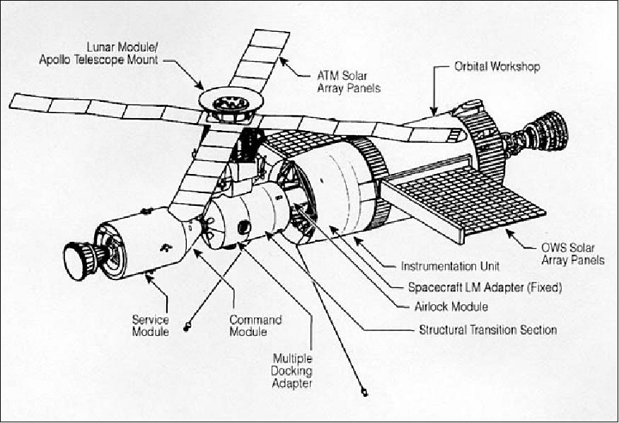
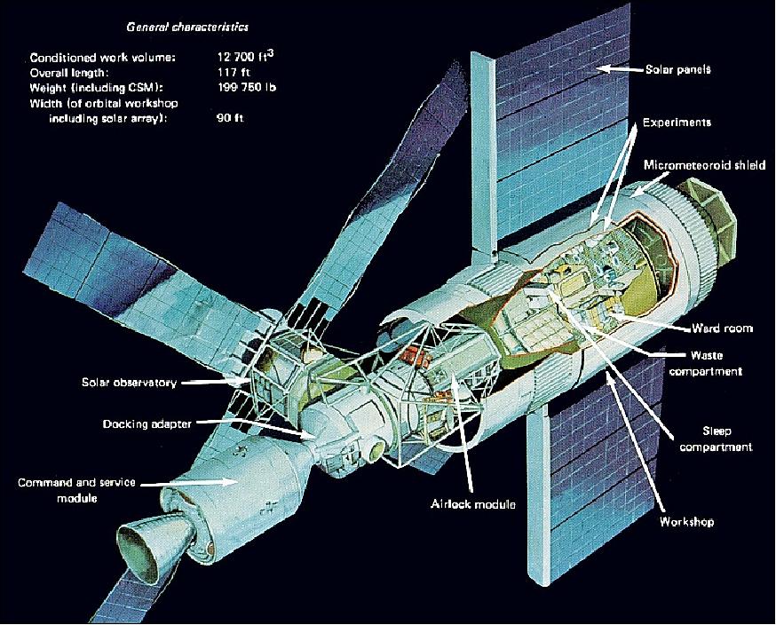
The Skylab spacecraft (space station) was composed of five elements or modules (assembled from leftover Saturn 5 and Apollo hardware components - originally intended for one of the canceled Apollo Earth orbital missions):
ATM (Apollo Telescope Mount)
The ATM was attached to one end of the cylindrical workshop. It was used to study the sun, stars and Earth with no atmospheric interference. ATM had a length of 3.4 m and a diameter of 2.1 m.
MDA (Multiple Docking Adapter)
The MDA permitted more than one Apollo spacecraft to dock to the Skylab station at once. MDA had dimensions of 5.2 m in length and 3.2 m diameter.
AM (Airlock Module)
The AM used by the Astronauts to access the outside of Skylab for spacewalks. AM had a length of 5.4 m and a diameter of 3.1 m.
IU (Instrument Unit)
The IU facility was designed by NASA/MSFC and used by NASA teams in Huntsville to reprogram the space station using a massive ring of computers (IBM). The unit was used to guide Skylab itself into orbit. IU also controlled the jettisoning of the protective payload shroud and activated the onboard life support systems, started the solar inertial attitude maneuver, deployed the Apollo Telescope mount at a 90º angle and deployed Skylab's solar panels. IU length of 0.9 m and a diameter of 6.6 m.
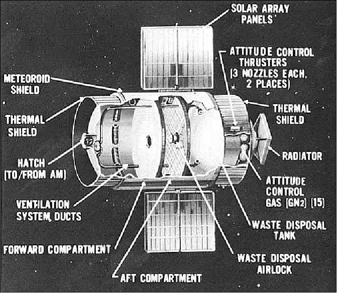
OWS (Orbital Workshop)
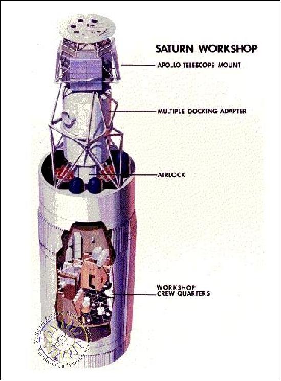
The OWS was the living and working area for the crew of three astronauts. OWS had dimensions of 14.7 m length and 6.7 m diameter. Attached to the outside wall of OWS are two large, wing-like solar arrays. The interior of this stage, which originally consisted mainly of two tanks for liquid hydrogen and liquid oxygen, underwent thorough conversion; the larger hydrogen tank became a living and working facility (the Workshop) for three astronauts, and the smaller oxygen tank became a container for waste products accumulating during the mission.
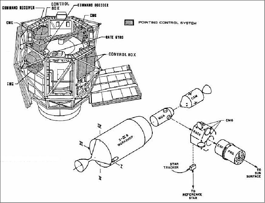
The Skylab structure was in the form of a cylinder, with the ATM being positioned 90º from the longitudinal axis after insertion into orbit. The ATM was a solar observatory; in addition, it provided attitude control and experiment pointing for the rest of the cluster. It was attached to the MDA and AM at one end of the OWS. The retrieval and installation of film used in the ATM was accomplished by astronauts during extravehicular activity (EVA). 1) 2) 3) 4) 5) 6) 7) 8)
The MDA served as a dock for the command and service modules, which served as personnel taxis to the Skylab. The AM provided an airlock between the MDA and the OWS, and contained controls and instrumentation. The IU, which was used only during launch and the initial phases of operation, provided guidance and sequencing functions for the initial deployment of the ATM, solar arrays, etc. The OWS was a modified Saturn 4B stage suitable for long duration manned habitation in orbit. It contained provisions and crew quarters necessary to support three-person crews for periods of up to 84 days each. All parts were also capable of unmanned, in-orbit storage, reactivation, and reuse.
Skylab size: 26 m length and about 6.7 m in diameter, the total mass was about 84,700 kg (about 283 m3 for living space, divided onto two floors; one floor was used for storage, conducting experiments and exercise equipment, including a static bicycle and treadmill; the second floor provided living quarters, including shower and dining facilities and a work area). With the docked Apollo command and service module, the assembly had a total length of 36 m and a mass of about 90,600 kg (90.6 tons). 9)
Launch
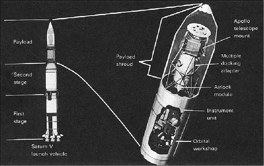
The launch of the unmanned Skylab spacecraft (i.e., Skylab-1) took place on May 14, 1973 from KSC (Kennedy Space Center, FLA) by a two-.stage version of a Saturn 5 rocket (the last Saturn 5 to be launched from pad 39A), replacing the 3rd stage (the Saturn-4B booster had been transformed into an orbiting workshop). Skylab-1 was launched in one launch and required no on-orbit assembly.
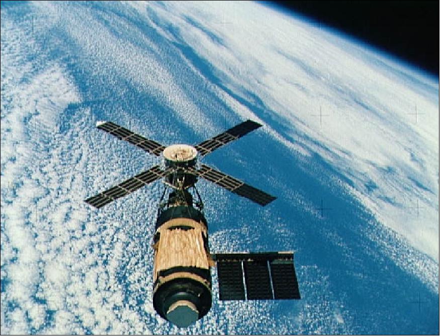
During the ascent phase, Skylab-1 experienced some damages. At 63 seconds after liftoff, the telemetry indicated a shield deployment and separation of the two major solar panels of Skylab-1. The objective of the shields was to provide Skylab with micro-meteoroid and thermal protection. The shields had vibrated loose and were ripped off by atmospheric drag, damaging one of the solar panels (or solar array wing) which partly deployed, and leaving debris which prevented deployment of the second solar panel.. Skylab-1 had, however, achieved its intended orbital altitude. Without the shield temperatures in Skylab soared to 52ºC.
As a consequence, the launch of the first crew, who was to occupy Skylab-1 the following day, was delayed for 10 days to arrange for proper replacements of four hardware systems - intended to combat the Skylab temperature problems caused by the loss of the shield. Also, the Skylab CMG (Control Moment Gyro) and PCS (Pointing and Control System) had to be reconfigured to accommodate the significantly altered moments of inertia and to adjust the control systems gains accordingly. 10)
Skylab was subsequently visited by three Apollo astronaut crews (using the Apollo Command and Service Module (CSM) launched on the less powerful Saturn S-1B booster), who lived and worked in the laboratory for periods of 28, 59, and 84 days respectively (1st crew launch: May 25, 1973 to Feb. 8, 1974 (last splashdown of a crew). Each crew return flight made use of the CSM.
Once on board, the first astronaut crew put a temporary parasol-type heat shield (sunshade) on Skylab which brought the temperature down to almost normal. However, most operations were prevented by the shortage of power. The astronauts made a three and a half hour space walk to fix the solar panels. During this EVA, they used a pair of wire cutters at the end of a 8 m long pole to cut the strap of metal that was holding the panel shut. Once out of the way, the solar panel was deployed and the station soon had enough power and the workshop became habitable.
Further repairs by subsequent crews led to virtually all mission objectives being met. The effectiveness of Skylab crews exceeded expectations, especially in their ability to perform complex repair tasks. They demonstrated excellent mobility, both internal and external to the space station, showing astronauts to be a positive asset in conducting research from space (Ref. 6).
Mission | Launch date | No of Earth orbits | Return flight of crew |
Skylab-1 | May, 14, 1973 (unmanned) | 34,981 (total) | July 11, 1979 (reentry) |
Manned missions to Skylab-1 | |||
Skylab-2 | May 25, 1973 (manned) | 404 (28 days) | June 22, 1973 |
Skylab-3 | July 28, 1973 (manned) | 858 (59.5 days) | Sept. 25, 1973 |
Skylab-4 | Nov. 16, 1973 (manned) | 1,214 (84 days) | Feb. 8, 1974 |
Orbit
Near-circular orbit, altitude = 435 km, inclination = 50º, period = 93.4 minutes.
Mission Updates
Skylab reentry: After hosting three teams of astronauts, the unmanned Skylab-1 was left in a stable orbit (and attitude) and systems were shut down. It was expected that Skylab-1 would stay in orbit for another 8-10 years. However, in 1977 it was discovered that its orbit was beginning to decay prematurely due to increased solar activity causing an expansion of Earth's atmosphere. This resulted in increased drag. Skylab-1 reentered the Earth's atmosphere on July 11, 1979, breaking up in the upper atmosphere with fragments scattering (some fiery debris) over the Indian Ocean and parts of sparcely-populated western Australia. The reentry generated a lot of press coverage for several months (alarming people and government agencies around the world).
Spacecraft
Attitude and Control of Skylab
The original mission for which Skylab was designed was to point at the sun and to gather scientific information. In addition, mission requirements called for pointing to various stellar targets and to nadir for Earth resources experiments. Several types of attitude sensors were used on Skylab. Many of the experimental instruments had their own fine attitude sensing and control apparatus that was designed to meet that experiment's needs. For example, the scientific cannister in the ATM needed to point at the sun with extreme accuracy. Provided with a course alignment towards the sun by Skylab, the experiment pointing control system used redundant precise Sun sensors and four rate-integrating gyros to sense and update the experiment attitude. These were mated through an analog computer to control actuators consisting of a manual pointing controller, pitch-and-yaw flex pivot actuators, and a roll positioning mechanism to correct experiment pointing. These actuators provided 120 degrees of roll motion and 2 degree motion in the pitch and yaw axes. Stability of up to 1 arcsecond of drift in 15 minutes was provided by this system. 11) 12) 13)
Skylab featured a sun seeker mounted in the ATM, designed to remain pointing towards the center of the sun, giving the Skylab module a reference vector to the sun. This location was chosen since one of the principle objectives of Skylab was solar study. In addition, there was a star tracker for attitude sensing (however, it experienced a lot of problems on all manned Skylab missions).
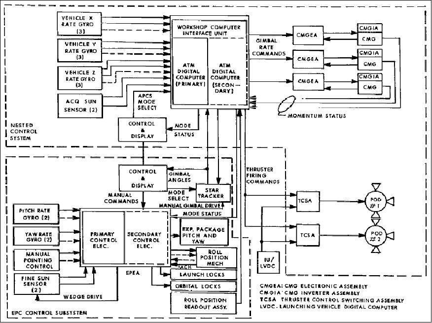
Skylab actuators
• Conventional rate gyros (9, 3 per axis), mounted in ATM, were used to measure the moments about Skylab's principle axis.
• The TACS (Thruster Attitude Control System) on Skylab consisted of six nitrogen gas expulsion nozzles mounted on the aft ent of the Orbital Workshop arranged in two 3 engine clusters on opposite sides of the Workshop. The TACS was used to control Skylab during spin-up of the CMG rotors during the first 10 hours of each mission, docking with the CSM, and as a backup system (dumping of CMG momentum). TACS was being used as a secondary control system to conserve fuel.
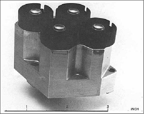
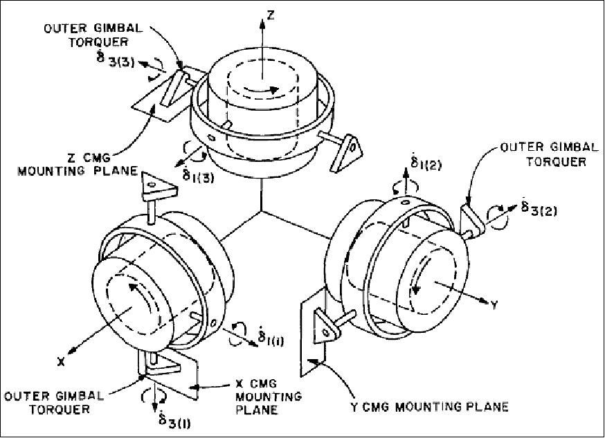
• CMGs (Control Moment Gyros) were introduced for the first time on a spaceborne platform for primary attitude control of a long-term mission (Note: a CMG is a gyroscope large enough to impart controlling moments or torques directly to a spacecraft; they are also referred to as "momentum exchange" or "momentum storage" devices). Three mutually orthogonal CMGs, each with a rotor diameter of 53 cm, and a mass of 65.5 kg, were installed to provide attitude control for the Solar Observatory in the ATM during solar observations. The instrument had to be pointed within 2.5 arcseconds of the desired direction and held there without drifting more than 2.5 arcseconds in 15 minutes' time.
Each CMG was a double-gimbal-mounted unit, electrically driven with a nominal spin of 9100 rpm, and capable of providing an angular momentum of 315 Nms. This CMG system was capable only of coarse pointing - within 6 arcmin (or 0.1º), two orders of magnitude larger than the instruments required. Mechanical constraints limited the travel of the CMG gimbals; and after a long period of absorbing unwanted torques, the CMG rotors reached a position of saturation. Hence, desaturation (or momentum dumping) took place in periods of no observation using TACS.
• An order of magnitude more stable pointing was needed for the ATM solar observatory. This was accomplished with the solar PCS (Pointing Control System). PCS was designed to point the entire ATM at any desired angle in pitch and yaw relative to the solar center. The accuracy of PCS was ±1.25 arcsec, the signal was sent to the torque motors that controlled the rotational positions of the ATM canister gimbals. The pointing coordinates were displayed on the C&D (Control and Display) panel for use by the crewman, they were also transmitted to the ground - and they were recorded on the ends of the film strips of the S-082A and B by photography of a photodiode matrix built into each of these instruments.
EPS (Experiment Pointing System). EPS is a two-axis gimbled system which being used as a fine pointing system for directing the experiment package on the ATM. The requirements call for a maximum range of ±3.5 x 10⁻² rad. The primary requirement for the EPS is to provide experiment package isolation from the relatively large vehicle perturbations that can result because of astronaut motion effects.
Overall, the APCS (Attitude and Pointing Control Subsystem) consists of the three basic systems: the CMG, the TACS, and the EPS. The first two systems may control the Skylab either separately or together in a nested configuration. The EPS system is used only for experiment spar control.
The EPS operates independently from the CMG system and TACS. It has its own sun sensors and rate gyros for position and rate control. Control signals are generated in theEPEA (Experiment Pointing Electronic Assembly), an analog device.
RF communications: Communications for the Skylab mission were handled through the Spacecraft Tracking and Data Network (STDN). This ground based system consisted of 13 sites during the Skylab mission. Real-time telemetry was limited to about 32% of the total time with a contact time averaging 6.5 minutes per site.
The communications hardware was focused in three systems to provide redundancy in case of failure. One system was in the Command and Service Module that brought the astronauts up to Skylab. This system was composed of a unified S-band transponder with a Pulse Code Modulating (PCM) system. Voice communications with the ground were carried out through the CSM communications system. Periodic television transmission from the 5 Apollo Telescope Module cameras and the portable cameras were routed through the S-band as well. Data storage for return to Earth and for some dumping was also conducted through the CSM. For rendezvous with Skylab, a VHF system was used to transmit a tone-modulated signal to Skylab where a corresponding transponder would receive and then retransmit the signal back to the CSM. The phase difference would then be measured to compute the relative distance and closing rate between Skylab and the CSM. - Another system was mounted in the Apollo Telescope Mount (ATM) and consisted of a VHF transmitter and UHF command receiver/decoder. Again, a PCM system was used. Data storage and subsequent dumping was carried out through this system as well as total control of the ATM by the crew.
The third system was located in the Airlock Module (AM). It also consisted of a VHF transmitter and UHF digital command receiver with a PCM. Data storage and dump could also be carried out through here. One of the innovations of Skylab was the use of a teleprinter to communicate with the crew.
Skylab power generation: The power generation was performed by two independent subsystems, one based on the ATM and one on the OWS. Each subsystem's solar arrays had an area of approximately 110 m2 and had a gross production of about 12 kW. The conditioning and battery systems reduced the output to about 4 kW each. The two power systems were interconnected in parallel to allow maximal utilization of available power. The total demands on the system ranged from 3.2 kW during unmanned periods to an average of 5.8 kW during occupation.
EREP (Earth Resources Experiment Package) sensor complement
From the large number of experiments onboard Skylab, only the EREP (Earth Resources Experiment Package) and solar observation experiments/instruments are described here (for instance, there were also a number of investigations in the areas of space science and astronomy). The overall objective of the EREP was to test the use of sensors that operated in the visible, infrared, and microwave portions of the electromagnetic spectrum to monitor and study Earth resources. A secondary objective of EREP was to determine what kind, and how much, photographic data (analog film) could be acquired of the broad variety of Earth features observed on the mission's ground track. EREP was conceived and operated as a facility, with data from all sensors freely available to PIs on all approved experiments. 14) 15)
Skylab was unique in that the presence of man made it possible to use photographic film as the prime detection and recording media for a variety of optical instruments and experiments. A large number of film rolls were used to support over thirty experiments and crew operational photography. The multi-discipline application of photographic film on Skylab provided invaluable information on the use and storage of film in space. The environmental impact on these films became an important consideration in the overall performance of the optical sensors. 16)
Background
It should be noted that the CCD (Charge Coupled Device) detector technology was still in its very infancy in the early 1970s. No CCD camera had been flown so far, airborne or spaceborne. While the technology of solid-state charge-transfer detectors was invented in 1969, it took until 1976 when the first astronomical ground observation with a CCD was done at the Mount Bigelow observatory of the University of Tucson, AZ; and the first experimental airborne instrument featuring a pushbroom CCD line detector, EOS (Electro-Optical Scanner) of DLR, was flown in early 1978.
Instrument naming nomenclature
Most Skylab instruments were labeled uniformly with an S (for Skylab) and a three-digit number.
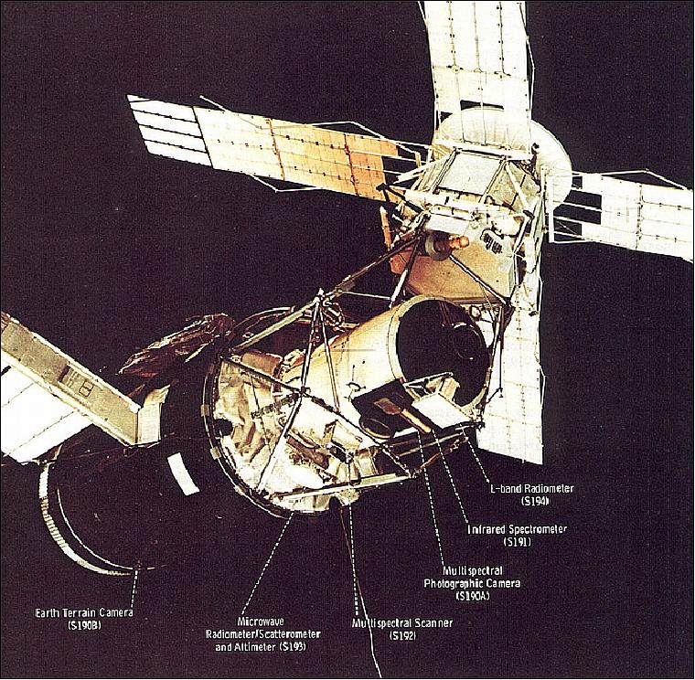
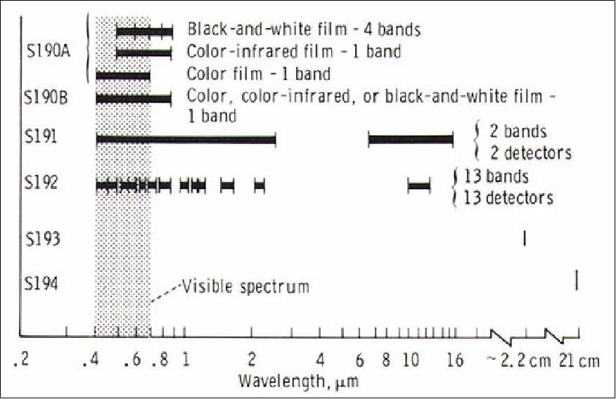
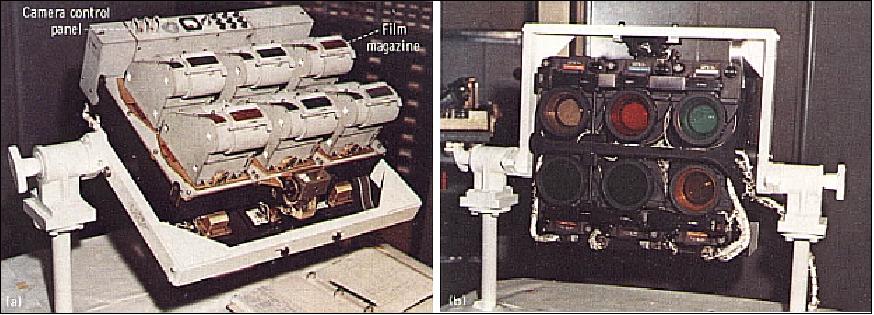
S-190A (Multispectral Photographic Camera System)
S-190A used six identical cameras with different film/filter combinations in order to view the same ground area simultaneously in the visible region. The S190A experiment consisted of 6 high-precision 70 mm cameras. The matched distortion and focal length camera array contained forward motion compensation to correct for S/C motion. The f/2.8 lenses, with a focal length of 15.2 cm, had a FOV of 21.1º providing a surface coverage of about 163 km x 163 km (image). The system was designed for the following wavelength/film combinations: 1) 0.5-0.6 µm, Panatomic-X B+W; 2) 0.6-0.7 µm, Panatomic-X B+W; 3) 0.7-0.8 µm, IR B+W; 4) 0.8-0.9 µm, IR B+W; 5) 0.5-0.88 µm, IR color; and 6) 0.4-0.7 µm, high-resolution color. The spectral regions designated were selected to separate the visible and photographic infrared spectrum into bands that were expected to be most useful for multispectral analysis of earth surface features. Further spectral refinements were made by using different filter combinations. The camera system provided photos with a ground resolution of 30 to 46 m in the visible wavelengths and 73 to 79 m in the infrared wavelengths.
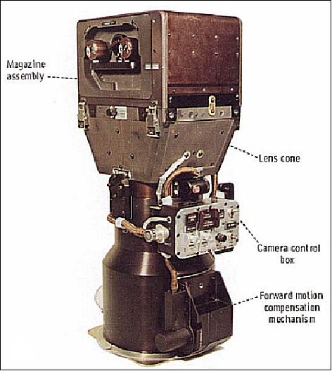
S-190B (Earth Terrain Camera)
Objective: Obtain high resolution data of small areas to aid interpretation of data gathered by EREP remote sensors. The PI was K. J. Demel, NASA JSC, and the contractors were: Actron Industries, Inc., Monrovia, CA; North American Rockwell, El Segundo, CA. The S-190B camera utilized a single 45 cm focal length lens with 12 cm film. Its field of view of 14.2º provided a surface coverage of about 109 km x 109 km. This camera was designed to use high-resolution color film and was operated from the OWS window, producing photos with a ground resolution of 17 to 30 m. The camera compensated for S/C forward motion through programmed camera rotation. Shutter speeds were selectable at 5, 7, and 10 msec with a curtain velocity of 2.8 m/s.
S190A Camera System | S190B Camera System | ||
Spectral range: | 400 - 900 nm | Spectral range | 400 - 880 nm |
Focal length: | 152 mm | Focal length | 457 mm |
Image format: | 5.7 x 5.7 cm | Image format | 11.4 x 11.4 cm |
Image scale: | 1 : 2,850,000 | Image scale | 1 : 950,000 |
Image overlapping: | 60% | Image overlapping: | 60% |
FOV | 21.2º | FOV | 14.24º |
Image size | 163 x 163 km | Image size | 109 x 109 km |
Ground resolution | 100 - 260 m | Ground resolution | 55 - 100 m |
Note: The S-190 camera systems are also known by the name of "multispectral photo facility," they were provided by ITEK.
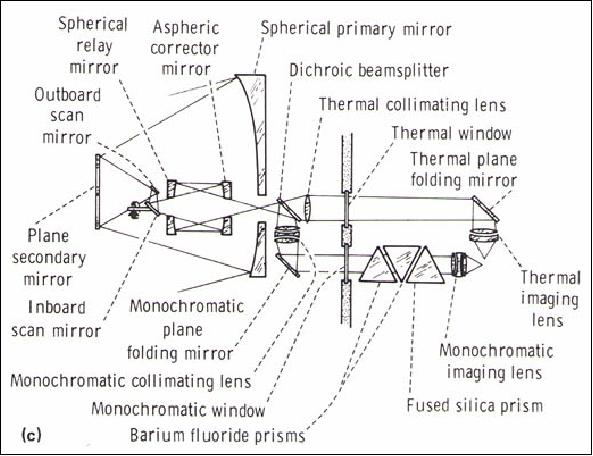
S-191 (Visible-Infrared Spectrometer)
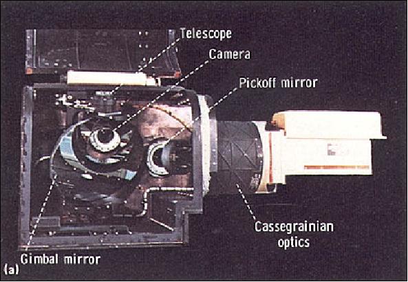
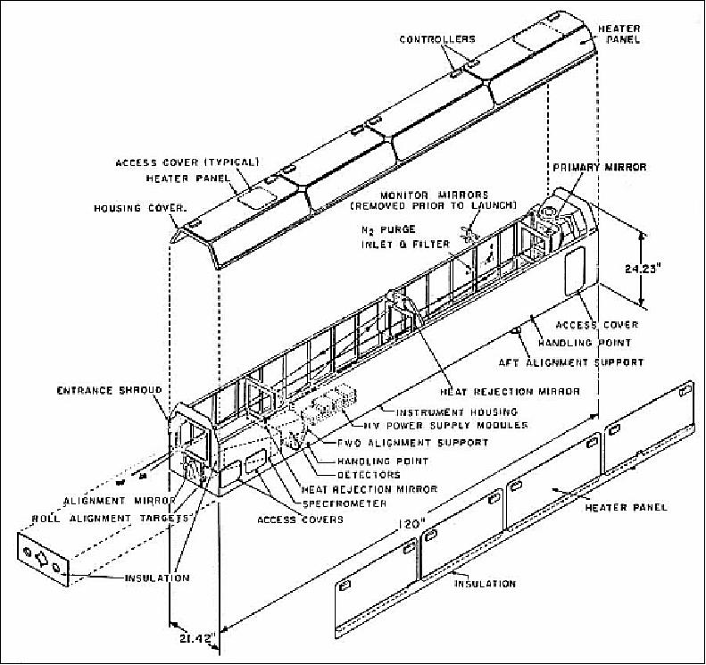
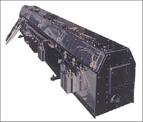
The objective of the S-191 camera system is to make an evaluation of the applicability and usefulness of sensing Earth resources from orbital altitudes in the visible through near-infrared and in the far infrared spectral regions (complement to the S-192 multispectral scanner). The S-191 experiment was basically a two-channel visible and infrared spectroradiometer (manually pointed device), consisting of the electronics module, the spectrometer module, and the calibration module. Measurement of radiation flux in the bands from 0.4 - 2.4 µm (reflective flux), and from 6.2 - 15.5 µm (emissive flux). FOV = 1 mrad (0.435 km diameter circular foot print), with a spectral resolution of 1 to 5%. 17) 18)
There were three detectors in the spectrometer. In the thermal channel, a HgCdTe detector enclosed in a dewar, was cooled to about 95 K by a miniature closed-cycle refrigerator. In the short wavelength channel, there was a sandwich detector: silicon in the range 0.4-1.1 µm, and lead sulfide (PbS) in the range 1.0-2.5 µm. The calibration module was placed in front of the aperture of the spectrometer. Three radiance sources rotated into position to fill the FOV: a heated black source, an ambient black source, and the cap of an integrated sphere, having an incandescent bulb, illuminated it. The latter source was for the VNIR channel, the former two were for the thermal channel. The calibration sequence was stepped through automatically, taking 2.5 minutes.
Note: The S-191 and S-192 experiments were operated from May 1973 to Feb. 1974. Both systems provided useful data. The data return was limited by the amount of magnetic tape that could be transported in resupply flights.
S-192 (Multispectral Scanner)
S-192 is a 13-band optomechanical instrument developed by Honeywell, Lexington, MA (PI: C. L. Korb, NASA/JSC). Objectives: to assess the feasibility of multispectral techniques, developed in the aircraft program, for remote sensing of Earth resources from space. Specifically, attempts were made at spectral signature identification and mapping of ground truth targets in agriculture, forestry, geology, hydrology, and oceanography.
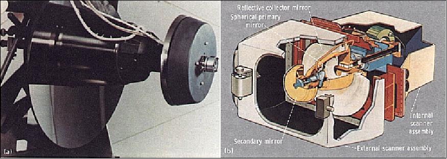
The S-192 optomechanical scanner utilized a 30 cm reflecting telescope with a rotating mirror in the image plane. The telescope and mirror were mounted outside the multiple docking adapter. Spectral range: 0.4-12.5 µm; number of spectral bands = 13; use of silicon detectors for bands 1-12 (0.41 - 2.43 µm), while band 13 (10.2 - 12.5 µm) used photoconductive HgCdTe detectors; radius of circular scan = 42 km; swath width = 72.4 km; IFOV = 79 m (0.182 mrad.); instrument mass = 57 kg; power = 266 W (peak).
The conical scan pattern was formed by giving the scanner a 9º forward tilt from nadir. Scanning was accomplished by a small flat fold mirror rotating on an arm to scan a circular zone of the image in the first focal plane of the telescope (primary spherical mirror of 51 cm diameter). The scan mirror scanned a zone of this known constant spherical aberration and subsequently corrected by the refocusing optics.
The 0.182 mrad IFOV measured by each detector provided an instantaneous ground coverage of a square area 79 m. Although the scan assembly rotated a full 360º, only the forward 110º were used to obtain surface data with the calibration data taken on the remainder of the scan. The corresponding sweep angle viewed from the sensor was 10.4º, which provided a swath width of 72.4 km.
Since the original thermal detector (Y-3) had less than the specified sensitivity, a more sensitive detector (X-5) was installed in January 1974 during the Skylab 4 mission. The checkout of this instrument was accomplished January 15 to 17, 1974.
Band No | Spectral Range (µm) | Comment (color) |
1 | 0.41 - 0.46 | Violet |
2 | 0.46 - 0.51 | Violet blue |
3 | 0.52 - 0.56 | Blue-green |
4 | 0.56 - 0.61 | Green-yellow |
5 | 0.62 - 0.67 | Orange-red |
6 | 0.68 - 0.76 | Deep red and infrared |
7 | 0.78 - 0.88 | Near infrared |
8 | 0.98 - 1.08 | Near infrared |
9 | 1.09 - 1.19 | Near infrared |
10 | 1.20 - 1.30 | Near infrared |
11 | 1.55 - 1.75 | Middle infrared |
12 | 2.10 - 2.35 | Middle infrared |
13 | 10.20 - 12-50 | Thermal infrared (TIR) |
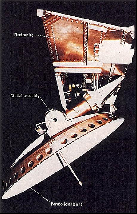
S-193 (Passive Microwave/Active Scatterometer and Radar Altimeter)
The radiometer/scatterometer portion of the instrument was also referred to as RADSCAT. The instrument was designed and developed at General Electric (prime contractor, PI: D. Evans, NASA/JSC). Objectives: simultaneous measurements of radar backscatter and radiometric brightness temperature in a number of scanning modes, primarily for the purpose of studying surface winds and precipitation over the oceans, and to provide engineering data for use in designing space radar altimeters. 19) 20) 21) 22) 23) 24)
The instrument design represents a first implementation of a combined passive/active microwave sensor. All three instrument components operated at the same frequency of 13.9 GHz (Ku-band) and microwave parts of the receiver, and shared a common gimballed antenna (mounted on the outside of the multiple docking adapter) and scan system. At the intermediate frequency, the received signal could go to one of three sections: wide band for the radiometer, somewhat narrower band for the altimeter, and narrow band for the scatterometer. The pulsed altimeter transmitter and interrupted CW scatterometer transmitter were switched to the antenna at appropriate times.
Spatial resolution = 16 km (circular footprint at nadir); mechanically scanning parabolic antenna (1.15 m diameter reflector) with dual polarization and a 2º FOV (swath width = 180 km). The antenna was gimballed, permitting along-track and cross-track scanning. Using a pulse width of 0.1 µs this system was able to get a resolution of 15 m. It operated over short orbital segments only but it was able to demonstrate the measurement of coarse features of the marine geoid such as major ocean trenches.
The scatterometer measured the backscattering coefficient of ocean and terrain as a function of incidence angle ranging from 0 to 48º. The radiometer was a passive sensor which measured the brightness temperature, from a cell on the Earth's surface, as a function of incidence angle from the surface. The altimeter was a compressed-pulse radar system to measure average ocean-surface elevation variations with a resolution of about 0.9 m. The S-193 ground coverage was 48º forward and 48º to either side of the spacecraft ground track. Scanning was possible in several modes. For precise measurements, the beam was scanned in the along-track direction to fixed angles from vertical of 0º, 15.6º, 29.4º, 40.1º, and 48º, with sufficient dwell time at each angle to permit averaging enough to achieve better than 5% precision. This was the primary mode used over the ocean. Timing was such that a given surface patch was observed successively at each of the angles. A more rapid along-track scan permitted continuous coverage at lower precision, a requirement for land surfaces. Cross-track scanning was possible at each of the selected angles with the lower precision of the rapid along-track scan; the 29.4º angle (incidence at the ground about 35º) was widely used over land.
Note: Prior to Skylab, RADSCAT was test-flown over the ocean on a C-l30 Starlifter aircraft of NASA.
The S-193 instrument had only a single pencil-beam, and it was not rotated in such a way as to observe backscatter from the same locations on the ocean surface at different viewing geometries. Thus, only a single observation was typically obtained; independent information on wind direction was required to retrieve wind speed (or vice versa) from S-193 measurements. Nonetheless, the S-193 experiment demonstrated that centimetric backscatter from the ocean could be detected by spaceborne instruments at moderate incidence angles, and that the radar cross-section varied appreciably with both wind speed and relative wind direction.
Data from the scatterometer showed that the 14.6 GHz values over land were sensitive to vegetation cover, surface water, soil moisture, and physiography. All data were recorded on magnetic tape on one digitized channel. The radiometer/scatterometer data were recorded at 5.33 kbit/s, the altimeter data at 10 kbit/s.
RADSCAT was the first western Earth-looking radar scatterometer carried in space, setting the stage for the more operational systems that followed. The instrument collected much backscatter information over the oceans (and land). When compared with ocean wind data, these results clearly showed the ability to measure ocean-surface winds from space.
The design of the S-193 introduced to radar the use of a measurement technique already in use on radiometers. This approach is being used on all subsequent spaceborne scatterometers. Previous radars required SNRs (Signal-to-Noise Ratios) well above 0 dB to make meaningful measurements. Radiometers and radio telescopes operate with SNRs of as small as -50 dB by separately averaging the receiver output and a calibrated noise, and then subtracting the noise power from the receiver output to get the received signal. Applying this new technique to the radar permitted the scatterometer to achieve 5% precision with -13 dB SNR. The bandwidth that could be used was only 10 s of kHz compared with typical radiometer bandwidths of 100 MHz and more; hence, the extremely low SNRs that radiometers use could not be achieved. 25)
S-193 radar altimeter
The primary objective of the technology instrument was to serve a) as a source of experimental short-pulsed data to be used in the design of future spaceborne radar altimeters and b) to demonstrate the ability of spaceborne altimeters in the acquisition of geodetic contour and oceanographic information over selected target areas. 26) 27)
Background: NASA and DoD started the National Geodetic Satellite Program in 1964 as a joint activity. The goal of this program was to develop a world datum accurate to within ±10 m and to refine the description of the Earth's gravity field. An ad hoc advisory group was formed in 1966 to advice NASA on the potential application to the geosciences of the ability to make geodetic measurements to accuracies of ±1 m and ± 0.1 m. The Williamstown Conference Report of 1969 (Williamstown, MA) had recommended to fly an altimeter on Skylab. The instrument demonstrated clearly that there were bumps and troughs on the surface of the oceans.
The primary measurements accomplished by the altimeter were individual return waveforms, backscattered signal power, and the round-trip ranging time. Instantaneous point samples of the return waveforms were obtained by using 8 high-speed S&H (Sample and Hold) gates, while the average return power was recorded by an integrating peak-detector network. The 2-way ranging time for altitude measurement was determined by a hybrid tracking loop which also positioned the S&H gates. The S-193 altimeter hardware had five selectable modes of operation as shown of Table 5.
The system was designed for acquisition of sigma-zero (σº) data through the use of AGC (Automatic Gain Control) measurements and internal calibration procedures. Precise (!) knowledge of the satellite's orbit relative to the Earth's surface was used to separate distance variations due to perturbations in the ocean surface from satellite-to-Earth distance variations due to orbital effects.
Parameter | Value | |
Transmitter | TWT power | 1 kW (min) |
Receiver | IF center frequency | 350 MHz |
Pulse compression | Type | Binary phase code |
Signal processing | Altitude tracking loop type | Digital, 200 MHz logic |
Waveform sampling | No of sample and hold gates | 8 |
Data rate | 10,000 bit/s (max) | |
Antenna | 1.15 m parabolic dish (see Fig. NO TAG#) | |
Mode | Experiment | Purpose | Comment |
I | Waveform and altimetry | 1) Provide short-arc geodetic profiling | 1) Data obtained at nadir and at 0.43º off nadir to check system alignment |
II | Radar backscattering cross-section | 1) Measure sigma-zero at 0.43, 1.3, 2.7, 7.6, and 15.6º angles of incidence | 1) To point calibration of AGC system provided |
III | Signal correlation | Determine min decorrelation between return pulses as a function of surface conditions | Pulse pairs are transmitted with a spacing between adjacent pulse stepped through the following values: 819.25, 409.65, 153.65, 76.85, 19.25, and 1.05 µs |
V | 10 ns and pulse compression | 1) Test pulse compression concept under extended target scattering from orbital altitudes | 13 bit Barker code bi-phase modulation used to obtain equivalent 10 ns pulse width from 130 ns pulse. 10 ns non-compressed pulse width also transmitted |
Nadir align | Nadir seeker | Provide self-alignment capability | Concept based on rapid decrease in theoretical peak of the mean return power as the antenna scans off nadir |
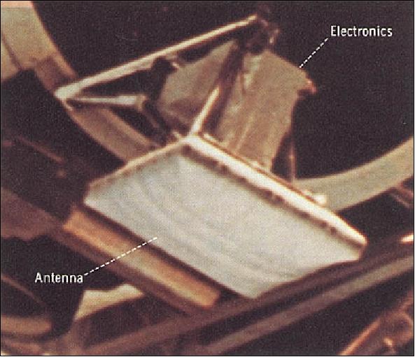
S-194 (Passive Microwave Radiometer in L-band)
S-194 was developed at Cutler Hammer Airborne Instrument Laboratory (PI: D. Evans of NASA/JSC). Objectives: to measure the microwave brightness temperature of the Earth's surface along the S/C track, to provide ocean surface features, varying winds over ocean areas, and Earth surface features information (soil moisture). S-194 was a modified Dicke-type radiometer with tuned RF receiver, gain modulation, and H polarization. Frequency = 1.4 GHz (21 cm wavelength); it utilized a fixed nadir viewing planar array antenna, recording thermal radiation at a frequency of 1.4 GHz and measuring the absolute antenna temperature. The system used a built-in calibration referenced to fixed hot and cold load input. The precision of the temperature measurement was 1 K.
The spatial characteristics were: an antenna half-power beam width of 15º, first null beam width of 37º (97% of power) and a circular footprint of about 124 km diameter (half-power). Data were recorded approximately three times per second, which resulted in a distance between centers of two consecutive resolution cells on the ground of 2.5 km. All data were recorded on magnetic tapes. The data output was at 200 bit/s.
S-063 (UV Airglow Horizon Photography)
The S-063 instrument was developed by NRL. The objective was to photograph the airglow, in particular at twilight, in several spectral bands within the VIS and mid-ultraviolet spectral range. A further objective was to study the Earth's ozone layer by vertical photography, using some of the airglow equipment. The airglow objectives were further modified after SL-3, the second manned mission, to include infrared photography of the OH (hydroxyl) airglow because of the availability of IR film and the need for wider passband photography of the airglow. 28)
Two 35 mm cameras were provided (Nikon adapted for Skylab), one for observations in the VIS spectral region with an F/1.2, 55 mm lens. The other camera was optimized for observations in the spectral range of 250-300 nm (mid UV) with an f/2 fused silica-calcium fluoride achromatic lens, also of 55 mm focal length. The UV and VIS cameras, the tracking sight, and a UV-transmitting solar SAL (Scientific Airlock) window were common to the ozone and airglow portions of the experiment. As the spacecraft traveled from sunset through night and into dawn. a line tangent to the airglow horizon rotated through 180º, becoming perpendicular to the Orbital Workshop (OWS) floor at midnight. Guidance of the camera was required of an astronaut during exposures of up to 64 s long. A tracking bracket was designed to move camera and guide telescope together as the astronaut maintained an illuminated rectile in position tangent to the VIS, unfiltered airglow band.
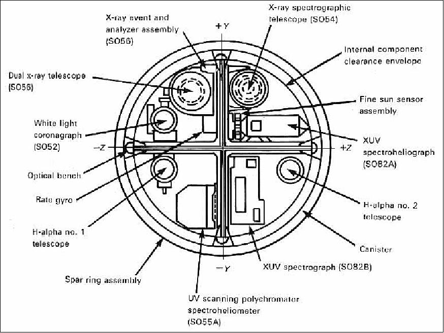
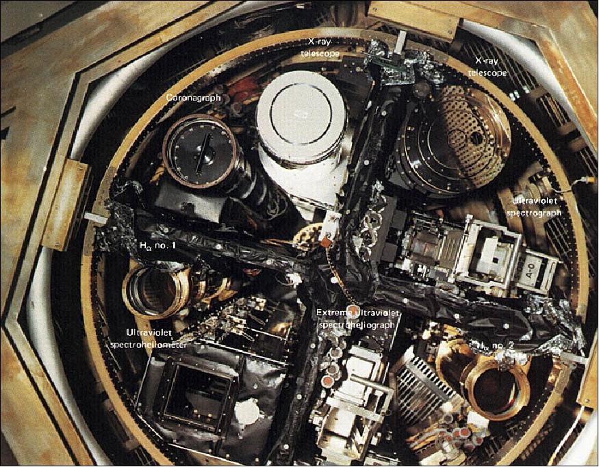
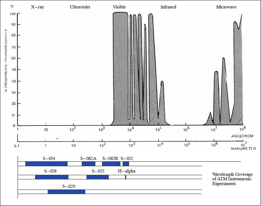
Solar payload complement
A main goal of Skylab was the study of the sun, in particular the corona with its flares and coronal transients, referred to as CMEs (Coronal Mass Ejections), in several wavelength regions not accessible from Earth. Several telescopes were available in ATM (Apollo Telescope Mount) to look at the sun in X-ray, ultraviolet, and H-alpha wavelengths, as well as in white light.
ATM on Skylab was the first full-scale, manned solar/astronomical observatory in space of the USA. The ATM canister [protective containment and instrument rack) was as large as any solar observatory spar on Earth at the time, measuring 3.36 m in length and 2.44 m in diameter (note: a "spar" is simply a box-like framework structure that is pointed towards sun)]. The solar telescopes on the ATM were not miniature models but full-sized observatory instruments, typically 3 m long and weighing, in all, more than 900 kg. Photoelectric sun sensors on the sunward face of the ATM canister provided error signals to large gyroscopes and actuators (CMGs) that were used to keep the entire ATM pointed at the sun to a tolerance of ± 2 arcsec.
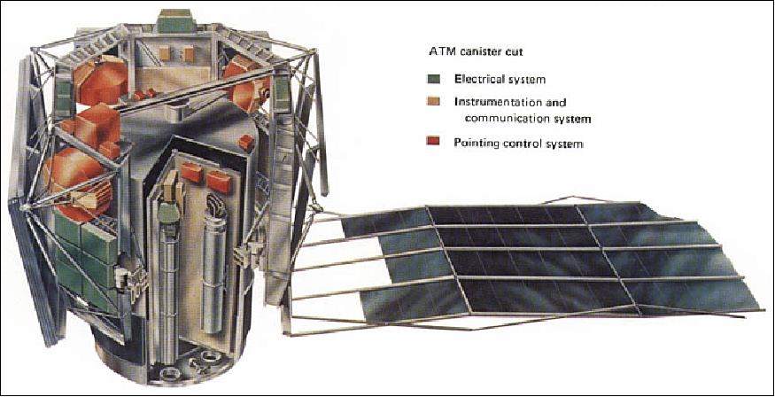
The ATM facility provided also vast capabilities for data recording in the early 1970 time frame. High-resolution film cameras were used to record the various instrument observations. The astronauts had the task to service (load and unload) the cameras and return the film at the end of their missions Earth. Nearly thirty film canisters were exposed and returned to Earth, providing scientists with over 150,000 exposures.
A single control and display console in the MDA (Multiple Docking Adapter) adjacent to the ATM permitted manual operation and visual monitoring of all the experiments on ATM through selector switches, pointing controls, TV monitors, and a variety of indicators of experiment status, film usage, solar conditions, and other parameters. The astronauts worked with the scientists on the ground, via radio exchange, in planning new programs and modifying others. They kept watch for flares and devised their own new ways of predicting flare occurrence.
Skylab included eight separate solar experiments on ATM consisting of the following instruments. Most of these solar instruments were descendants of instruments used in experiments flown on earlier, unmanned solar spacecraft. 30) 31) 32)
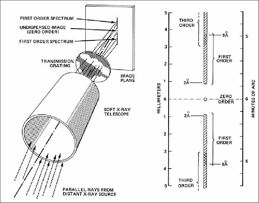
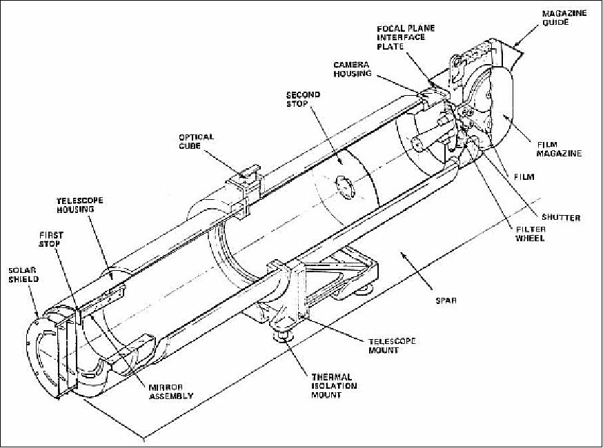
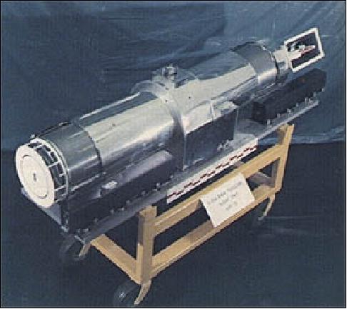
S-054 (X-ray Spectrographic Telescope)
S-054 was developed at AS&E (American Science and Engineering) Corporation, Cambridge, MA. The objective was to obtain X-ray images of the sun over a wavelength range from 0.2 to 6 nm (or 2 to 60 Å, 1Å = 10-10 m). Use of selective filters and a transmission grating to obtain spectral information.
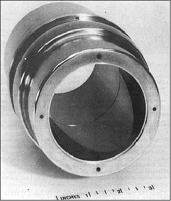
AS&E and GSFC jointly pioneered the use of the Wolter lens, grazing incidence telescope for imaging the sun in X-rays. The instrument provided a spatial resolution of approximately 2 arcsec on axis and had six broadband X-ray filters, each with a different transmittance curve. The instrument provided a spectrographic mode and an imaging mode. Each X-ray picture is accompanied by a white-light picture, co-aligned with the X-ray image. The data were recorded on film. Approximately 6500 frames of film were available on each film magazine. One camera magazine was used during the first manned (SL-2) Skylab mission. Two were used during the second mission (SL-3), and two magazines were exposed during SL-4. In total, approximately 32,000 solar X-ray exposures were obtained.
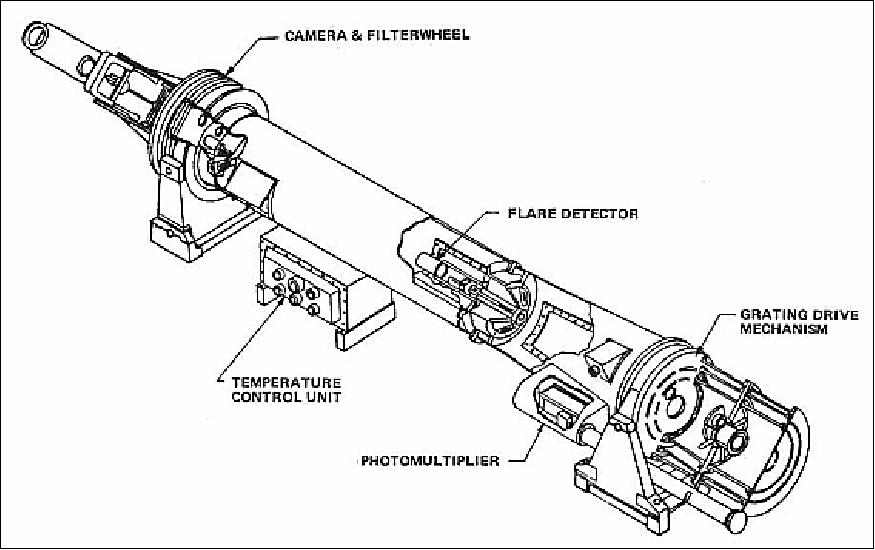
The telescope photographically records high-resolution images of the solar corona in several broadband regions of the soft X-ray spectrum. It includes an objective grating used to study the line spectrum. The spatial resolution, sensitivity, dynamic range and time resolution of the instrument were chosen to survey a wide variety of solar phenomena. It embodies improvements in design, fabrication, and calibration techniques which were developed over a ten-year period. The observing program was devised to optimize the use of the instrument and to provide studies on a wide range of time scales. 33)
This experiment included also a photomultiplier counter consisting of a NaI crystal of about 5 cm2 area and a covering window of 5.08 x 10⁻⁵ m of beryllium (Be). The counter operated in two modes: either the output went through a pulse-height analyzer, which provided 8 channels of counts from 10 keV to 80 keV, or the DC current was monitored and converted to a number proportional to the logarithm of the current.
S-056 (X-ray Telescope)
S-056 was a soft soft X-ray telescope designed and developed at NASA/MSFC. This grazing incidence telescope produced images of the sun in X-rays with wavelengths from 6 to 49 Å, together with an X-ray event analyzer to monitor the total solar soft X-ray flux in several wavelength bands. Images taken through 6 different filters were recorded on film which was then returned to Earth on return flights for processing. 34)
On a historical note, the S-054 and S-056 observations provided the first ever spaceborne X-ray imagery. These Skylab images clearly showed the utility of full-disk solar images for studies of coronal holes and solar flares. The synoptic record of solar coronal structure provided by these images has enabled researchers to discover trends in the lives of solar active regions, X-ray bright points, coronal streamers and other solar wind structures, as well as the evolution of the solar magnetic field over an eight-month interval. Originally these images were acquired in orbit on photographic film, and processed by printing slides and paper images. Years later, the micro-densitometer scans of the original film were made and stored on magnetic tapes.
In dimensions and general characteristics, S-056 and S-054 were much alike. The principle difference between them was that S-056 had three times less light gathering area, but was equipped with a different series of filters, which enabled it to record somewhat harder X-rays. S-056 was particularly successful in recording images of high spatial resolution, which showed the growth phase of solar flares in detail.
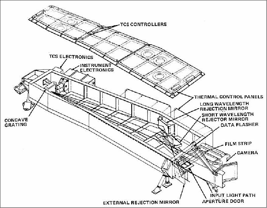
S-020 (XUV spectrograph)
S-020 was developed by NRL. The S-020 grazing incidence spectrograph is the only solar instrument located in the Orbital Workshop (OWS). The objective was to record on photographic film a spectrum of the X-ray and ultraviolet radiation from the sun in the 1-20 nm (or 10 - 200 Å) region, with modest angular resolution. Radiation in this spectral range is emitted by highly ionized atoms in the solar chromosphere and corona. This is indicative of high-temperature atomic and plasma processes which are extremely difficult to duplicate on Earth. 35)
Instrument: Sunlight entered a narrow slit and impinged upon a grating under a very small angle of incidence. Under conditions of grazing incidence, the gratings reflected sufficient energy even in the 1-10 nm wavelength region (soft X-ray region) to make film recordings feasible when long-time exposures could be made. Thin metallic films in front of the slit blocked out undesired ultraviolet and visible light.
Instrument | Instrument developer | Wavelength range | Solar region observed |
S-054 | AS&E Corp. Cambridge, MA | 2-60 Å | Corona (1 to 1.5 solar radii) |
S-056 | NASA/MSFC, Huntsville, ALA | 6-33 Å | Low corona |
S-020 | NRL, Washington, DC | 10-200 Å | Chromosphere, transition region, and low corona |
S-055 (EUV Spectroheliometer)
S-055 was developed by the Harvard College Observatory (HCO), Cambridge, MA. The S-055 instrument was a further development of similar instruments flown on OSO-4 (Orbiting Solar Observatory-4, launch Oct. 18, 19967) and OSO-6 (launch Aug. 9, 1969). 36)
The objective was to obtain photometric data of six spectral lines (O IV, Mg X, C III, O VI, H I, C II) and the Lyman continuum in the wavelength region from 30-140 nm from 5 x 5 arcsec surface elements of the sun. Also, to obtain a spectral scan of the 30-140 nm region by tilting the grating. The study of relative spectral line intensities provides information about plasma composition, temperatures, and energy transfer processes in quiet and active solar phenomena.
The instrument used an off-axis paraboloidal primary mirror to form a solar image on the entrance slit of the spectrometer of 56 µm x 56 µm in size, corresponding to an area of 5 arc sec x 5 arcsec on the sun. A diffraction grating with 1800 lines/mm produced a spectrum on the Rowland circle where seven photomultiplier detectors (Channeltrons) in fixed positions simultaneously recorded the intensities of the six lines and the Lyman continuum. Bi-axial motion of the primary mirror generated the desired raster scanning pattern (polychromator mode). 37)
In the grating scan mode, the primary mirror remained fixed while the grating is tilted to scan the entire operating spectrum past one or more of the photomultiplier detectors (7 detectors). The signals from the detectors were transmitted to the ground by telemetry.
The instrument was operated in both unattended and unmanned modes, but without the capability of fine pointing except when manned and the crewman in charge. Excellent results were obtained with the intensity data covering a wide dynamic range with high precision.
S-052 (White Light Coronagraph)
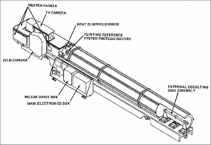
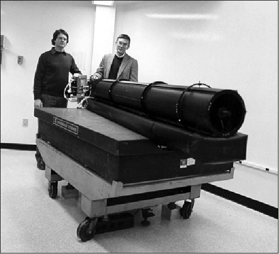
S-052 was designed by the High Altitude Observatory, Boulder, CO, and manufactured by Ball Brothers Research Corporation, Boulder,CO. The white light coronagraph was one of the principal ATM instruments for studying the sun's outer atmosphere, its corona. It was designed to photographically monitor the brightness of the solar corona over a wavelength range extending from 3500 - 7000 Å. The goal was to obtain high resolution, high sensitivity photographs of the solar corona from 1.5 to 6 solar radii (300,000 km to almost three million km) above the solar surface. Study of brightness, form, size, composition, polarization, and movements of the corona. Correlate the observations with solar surface events and with solar wind effects. 38) 39) 40)
Coronagraphs are designed to block out the image of the sun's disc and to take pictures of the faint corona which extends from the sun far into space. Light scattering by optical elements and by structural surfaces must be carefully avoided. This instrument contained four coaxial occulting discs and photodetectors for alignment corrections. Pictures were recorded on 35 mm film; they were taken either in unpolarized light or in one of three possible orientations of plane polarized light. Also, the instrument was able to operate in the "video mode" permitting a display for the astronauts or TV transmission to the ground.
S-052 operation took place in four photographic modes. In each mode, the shutter of the camera made three exposures of 0.5, 1.5, and 4.5 seconds duration. In the first mode, the triple exposure was made at each of the four different positions of the polarization filter wheel. In the second mode, the same sequence of 12 exposures was repeated continuously for 16 minutes. In the third mode, the triple exposures repeat was in fast sequence for 16 minutes, with the filter wheel in the "clear" position. The fourth mode was the same as mode three, except that a shutter opening occurred every 32 seconds only; this mode continued until manually stopped.
During the Skylab mission, the coronagraph obtained more than 35,000 broadband white-light photographs (370-700 nm) of the solar corona, both unpolarized and linearly polarized (the latter through Polaroid HN-38 filters). Five cameras, each loaded pre-mission with a 229 m long by 35 mm wide film roll, were recovered and replaced by astronauts on EVA maneuvers.
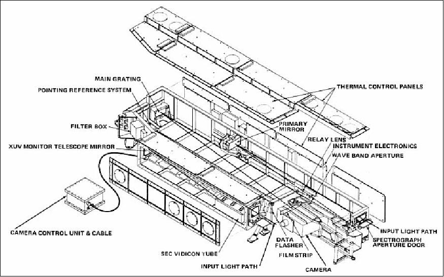
S-082A (XUV Spectroheliograph)
S-082A was developed by NRL (Naval Research Laboratory). S-82A was of an instrument heritage flown on OSO-2 (launch Feb. 3, 1965) and was outfitted with photomultiplier detectors. The objective was to record monochromatic images of the entire sun in the emission lines of a spectral range from 17 to 63 nm (extreme UV). Information was obtained about the composition, temperature, energy conversion and transfer, and plasma processes within the chromosphere and lower corona. These data were correlated with results from simultaneous observations in the other wavelength regions. Among the most intense lines in this extreme ultraviolet region are those of helium, oxygen, neon, magnesium, and iron. 41) 42)
The instrument was a slitless Wadsworth grating spectrograph using photographic recording. Imaging of the sun and generation of the spectrum was being achieved by a single concave mirror of 2 m focal length, ruled in gold with 3600 lines/mm (spectral range covered of 171-630 Å). Monochromatic, overlapping solar images of 18.6 mm diameter were being formed on a film strip. The instrument was designed to operate over two wavelength ranges with the grating normal located at 255 Å for the one and 400 Å for the other range (the two spectral ranges were being photographed separately, with two angular positions of the grating). The unused part of the solar spectrum was being reflected out into space in order to avoid unnecessary heating of the instrument. A thin aluminum filter in front of the film kept stray light out. Four film cameras, each loaded with 200 film strips, were being used.
S-082B (XUV Spectrograph)
S-082B was developed by NRL. The objective was to obtain XUV (Extreme Ultraviolet) spectra (97 to 394 nm or 970-3940 Å) of small portions of the solar surface with high spatial and spectral resolution, and to obtain photograph spectra at various locations on and off the disc and across the limb, from 12 arcsec below to 20 arcsec above the limb. Attempts were made to obtain spectra of flares and other active areas on the sun. Information on the change of the solar energy transportation mode from convection to plasma-dynamic shock waves was being derived from these observations. Also, details of structure, density, and temperature of the chromosphere and the lower corona were being studied. 43)
The instrument consisted of a single mirror telescope and a double grating spectrograph. The telescope mirror was an off-axis paraboloid of 1 m focal length and 54 mm x 121 mm clear aperture. The mirror formed on the entrance slit of the spectrograph a solar image of 9.3 mm diameter with a resolution of about 1 arcsec. A pre-disperser grating assembly with two gratings was being used to generate a light beam containing only the desired wavelength regions (elimination of stray light). The main grating, a concave mirror ruled at 600 grooves/mm, produced a spectrum on photographic film with a resolution of 0.004 nm in the 97 - 197 nm range and a resolution of 0.008 nm in the 194 - 394 nm range. The entrance slit admitted light from a 2 arcsec x 60 arcsec area on the sun. Image detection was done with photomultipliers. The photoelectric detection technology employed offered such features as increased precision of the intensity measurements and a wider dynamic range coverage over the photographic recording technique. To the greatest extent possible, the S-055, S-082A and S-082B instruments were operated together.
Instrument | Instrument developer | Wavelength range | Solar region observed |
S-082A | NRL, Washington, DC | 150-615 Å | Chromosphere, transition region, and low corona |
S-055 | Harvard College Observatory, Cambridge, MA | 300-1400 Å | Chromosphere, transition region, and low corona |
S-082B | NRL, Washington, DC | 970-3940 Å | Chromosphere, transition region, and low corona |
Hydrogen-Alpha Telescopes
The two instruments were developed by Harvard College Observatory (HCO) and by NASA/MSFC. The objective was to use two telescopes imaging the sun in the red light of the hydrogen-alpha line (Balmer series) to provide a visual aid to the astronauts and a photographic record of solar conditions during ATM solar observing periods (study of H-alpha emission from the sun during solar flares). 44)
The H-Alpha telescope consists of a telecentric Cassegrain objective (f/28) and relay optics. A 5.1 cm diameter image of the sun (6.4 cm on H-Alpha II) is formed in the focal plane and relayed to one of two image planes (vidicon or film camera) via a zoom lens and a fixed relay lens, respectively. The vidicon cameras displayed real-time solar detail to the crew on one of the two video monitors on the ATM console in the MDA (Multiple Docking Adapter). Each of the telescopes had a mechanically movable cross-hair: that of telescope I was being aligned with the boresight of Experiment S-055, that of telescope 2 with the boresight of Experiment S-082B. Alignment was being accomplished by crew members, using the solar limb in two right-angled directions as reference system.
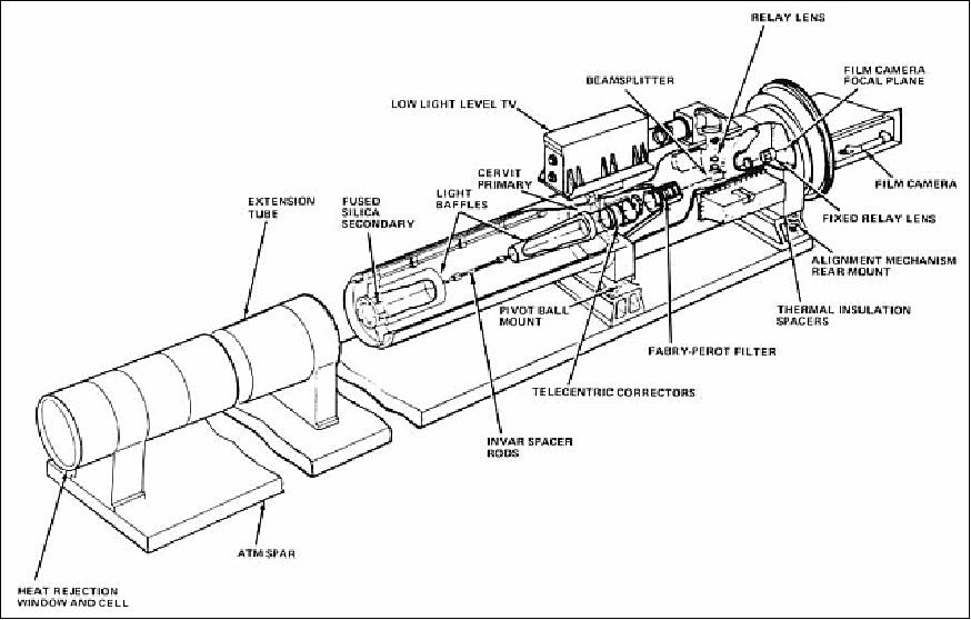
The hydrogen-alpha telescope 1 provided simultaneous photographic and TV pictures; its resolution was 1 arcsec at a field of view (FOV) of 4.5 arcminutes. Telescope 2 operated only in the TV mode, with a resolution of about 3 arcsec. Each telescope had a zoom capability, varying the FOV between 4.5 - 15.8 arcmin for telescope 1 and between 7.0 and 35 arcmin for telescope 2. Selection of the desired spectral line (656.28 nm) was accomplished with a Fabry-Perot filter which contained a solid glass flat with coated surfaces as interference gap.
Instrument | Instrument developer | Wavelength range | Solar region observed |
H-Alpha 1 | Harvard College Observatory | 6563 Å | Chromosphere |
H-Alpha 2 | NASA/MSFC | 6563 Å | Chromosphere |
S-052 | High Altitude Observatory, Boulder, CO | 3500-7000 Å | Outer corona |
Experiment | Scientific objective |
S-009 | Cosmic Ray flux measurement - nuclear emulsion detector |
S-019 | UV line spectra of young, hot stars and galaxies down to 1400 Å |
S-073 | Gegenschein and zodiacal light intensity and polarization. Measure the surface brightness and polarization of the night glow over a large portion of the celestial sphere in the visible light spectrum and determine the extent nature of the spacecraft corona during daylight |
S-149 | Mass, speed and chemical composition of interplanetary dust. Determine the mass distribution of micrometeorites in near Earth space. |
S-150 | Faint X-ray source survey. Survey a portion of celestial sphere for galactic X ray sources in the 0.2 to 10 KeV energy range. |
S-183 | UV Panorama Experiment - photometer for stellar spectrography and a wide-field imaging camera. Obtain wide field of view photographs of individual stars and extended star fields in the UV range. |
S-201 | Far-UV Electrographic camera to study Comet Kohoutek structure |
S-228 | Transuranic Cosmic Ray Experiment. Provide detailed knowledge of relative abundance and energies of the nuclei in cosmic radiation. |
Some pioneering Skylab achievements
Around 300 scientific and technical experiments were conducted onboard the Skylab space station in various fields including microgravity (crystal growth), medicine/space life sciences (test of the effects of long-duration space flights), biology, astronomy, and sun and Earth observations.
• More than 740 hours were spent in observing the sun by telescopes, and 175,000 solar pictures were returned to Earth, as were about 64 km of tapes. The retrieval and replacement of camera magazines required an EVA (Extra Vehicular Activity) by astronauts.
• The EREP (Earth Resources Experiment Package) of Skylab produced the first comprehensive and systematic image survey of the Earth from space. A total of 46,000 photographs were made of the Earth's surface. Much of the photography is archived at the EROS Data Center (representing a treasure as one of the earliest possible baselines from which to evaluate the environmental changes).
• An unanticipated major astronomical event caused revisions in planning for the third and final Skylab manned mission, the SL-4 mission. The passage of Comet Kohoutek was detected early enough in its trajectory permitting scientists to plan ahead for the most promising investigations. The third crew was able to perform a number of sightings of Comet Kohoutek.
• Skylab was a scientist's spacecraft: there were many sound experiments - and they were foremost in the mission. For the first time in space, there were few constraints on experiment mass, power consumption, telemetry, or film usage and storage. For the first time, solar astronomers were able to take advantage of photographic emulsions in long-term observational sequences in space. For the first time, repairs and modifications were made on experimental equipment during the operational phase of the mission - within Skylab and outside it, during spacewalks by astronaut crews. In this way, the first crew salvaged the entire mission. 45)
• The sensor complement (some of them prototype instruments) introduced several ground-breaking technologies for a spaceborne platform.
• The first spaceborne active sensors were radar systems on Skylab (the instrument was S-193, a combination of passive microwave radiometer with an active scatterometer, and radar altimeter) operated between May 1973 and Feb. 1974. This opened up the age of spaceborne microwave measurement of ocean winds, started with RADSCAT on Skylab (demonstration of the feasibility of scatterometer wind speed remote sensing). - Also, the first ever spaceborne monostatic altimetry measurements (demonstrations) of ocean surface heights started in 1973 with S-193. The availability of the S-193 altimeter data opened the way to a direct comparison of the altimeter heights with a computed gravimetric geoid.
• Initial experiments of marine wind measurements began with a scatterometer [S-193, the first spaceborne Ku-band scatterometer, also referred to as RADSCAT (Radiometer/Scatterometer)] on Skylab.
• The first ever spaceborne focussing X-ray telescopes (S-054, S-056) flew on Skylab and recorded over 35,000 full-disk images of the sun over a 9-month period (this represented also the first study of the sun the the X-ray range).
• Skylab computers: Skylab carried a highly successful computer system (quite a feat for the period of 1973 when practically no computers were flown onboard). It made a large contribution to saving the mission during the 2 weeks after the troubled launch and later helped control Skylab during the last year before re-entry. The entire system functioned without error or failure for over 600 days of operation, even after a 4-year and 30-day interruption. It is significant as the first spaceborne computer system to have redundancy management software. The software development for the system followed strict engineering principles, producing a fully verified and reliable real-time program.
• Skylab used for the first time the "off-the-shelf" IBM 4Pi series processors (Note: the Gemini and Apollo computer systems were custom-built processors). The 4Pi descended directly from the System 360 architecture of IBM developed in the early 1960s. The 4Pi model chosen for Skylab was the TC-1 (16-bit word length), adapted for use on Skylab by the addition of a custom input/output assembly to communicate with the unique sensors and equipment aboard the laboratory. A TC-l processor, an interface controller, an I/O assembly, and a power supply made up an ATMDC (Apollo Telescope Mount Digital Computer). Each TC-1 (there 2 on Skylab) had a memory of 16,384 words. 46)
• By using the computer system that controlled the workshop's attitude, the ground controllers were able to keep the Skylab at angles to the sun such that the equipment would be exposed to tolerable temperatures in the laboratory in concert with generating adequate power from the remaining solar panels.
• The first CMGs (Control Moment Gyroscopes), large-scale designs, were flown on Skylab to handle momentum management for a large space structure. Much later, the same CMG technology was also employed in the space stations MIR and ISS.
References
1) R. Tousey, "Apollo Telescope Mount of Skylab: an Overview," Applied Optics, Vol. 16, No 4, 1977, pp. 825-836
2) http://www.aerospaceguide.net/spacestation/skylab.html
3) http://solarscience.msfc.nasa.gov/Skylab.shtml
4) http://heasarc.gsfc.nasa.gov/docs/heasarc/missions/skylab.html#instrumentation
5) Kipp Teague, Steven J. Dick, Steve Garber, "Skylab Drawings and Technical Diagrams," URL: http://history.nasa.gov/diagrams/skylab.html
6) NASA Kennedy Space Center. URL: [web source no longer available]
7) W. David Compton, Charles D. Benson, "Living and Working in Space - A History," 1983, URL: http://history.nasa.gov/SP-4208/sp4208.htm
8) Roland W. Newkirk, Ivan D. Ertel, Courtney G. Brooks, "Skylab - A Chronology," NASA, 1977, URL: http://history.nasa.gov/SP-4011/contents.htm
9) U.S. Centennial of Flight. URL: [web source no longer available]
10) S. M. Seltzer, "The Saturn Launch Vehicle and its Guidance and Control (G&C) System)," Proceedings of the 27th AAS Rocky Mountain Guidance and Control Conference (J. D. Chapel, R. D. Culp, ed), Vol. 118, Feb. 4-8, 2004, Breckenridge, CO, pp. 409-426, AAS-04-061
11) "Skylab: A Guidebook," URL: http://history.nasa.gov/EP-107/ch4.htm
12) W. B. Chubb, S. M. Seltzer, "Skylab Attitude and Pointing Control System," NASA TN D-6068, Feb. 1971, URL: http://ntrs.nasa.gov/archive/nasa/casi.ntrs.nasa.gov/19710007043_1971007043.pdf
13) W. B. Chubb, H. F. Kennel, C. Rupp, S. M. Seltzer , "Flight Performance of Skylab Attitude and Pointing Control System," Journal of Spacecraft and Rockets, Vol. 12, No 4, 1975, pp. 220-227
14) Steven J. Dick, S. Garber, "SP-399, Skylab EREP Investigations Summary," URL: http://history.nasa.gov/SP-399/sp399.htm
15) R. L. Eason, "SP-399, Skylab EREP Investigations Summary, Appendix-A" URL: http://history.nasa.gov/SP-399/app-a.htm
16) L. P. Oldham, H. L. Atkins, "Photographic film and the Skylab environment," Applied Optics, Vol. 16, No 4, April 1977, pp. 1002-1008
17) P. Slater, "Remote Sensing," Optics and Electronics Systems, Addison-Wesley Publishing Co., 1980, pp. 456-462
18) T. L. Barnett, R. D. Juday, "Skylab S191 visible-infrared spectrometer," Applied Optics, Vol. 16, No 4, April 1977, pp. 967-972
19) E. G. Njoku, "Passive Microwave Remote Sensing of the Earth from Space," Proceedings of the IEEE, Vol. 70, No. 7, July 1982, pp. 728-750
20) J. D. Young, R. K. Moore, "Active microwave measurement from space of sea-surface winds," IEEE Journal of Ocean. Engineering, OE-2, pp. 309-.317, 1977
21) R. K. Moore, et al. "Simultaneous Active and Passive Microwave Response of the Earth - The Skylab RADSCAT Experiment," Proceedings of 9th International. Symposium on Remote Sensing of Environment, Ann Arbor, MI: University of Michigan, 1974, pp. 189-217.
22) F. T. Ulaby, R. K. Moore, A. K. Fung, "Microwave Remote Sensing: Active and Passive," Vol. 2, Artech House, Dedham MA, 1982.
23) R. K. Moore, W. L. Jones, "Satellite Scatterometer Wind Vector Measurements - the Legacy of the Seasat Satellite Scatterometer," IEEE Geoscience and Remote Sensing Society Newsletter, Cumulative Issue #132, September 2004, pp.18-32, ISSN 0161-7869
24) R. K. Moore, "Simultaneous active and passive microwave response of the Earth: The Skylab RADSCAT experiment," Proceedings of 9th International Symposium on Remove Sensing of the Environment, Ann Arbor, MI, 1974, Vol. I, pp.189-217
25) R. E. Fischer, "Standard Deviation of Scatterometer Measurements from Space," IEEE Transactions on Geoscience Electronics, Vol. GE-9, pp. 216-221, 1971.
26) J. T. McGoogan, L.S. Miller, G. S. Brown, G. S. Hayne, "The S-193 Radar Altimeter Experiment, Satellite Altimetry Applications, Proceedings of the IEEE, Vol. 62, No 6, June, 1974, pp. 793-803
27) L. S. Miller, D. L. Hammond, "Objectives and capabilities of the Skylab S-193 altimeter experiment," IEEE Transactions on Geoscience and Electronics (Special Issue - Third Annual International Geoscience Symposium - Selected Papers), Vol. GE 10, Jan. 1972, pp.73-79
28) D. M. Packer, I. G. Packer, "Exploring the Earth's atmosphere by photography from Skylab," Applied Optics, Vol. 16, No 4, April 1977, pp. 983-991
29) http://history.nasa.gov/SP-4208/ch4.htm
30) EP-107 Skylab: A Guidebook, Chapter V: Research Programs on Skylab, URL: http://history.nasa.gov/EP-107/ch5.htm
31) SP-402 A New Sun: The Solar Results From Skylab, The Solar Telescopes on Skylab, http://history.nasa.gov/SP-402/ch4.htm
32) http://wwwsolar.nrl.navy.mil/skylab_atm.html#skylab
33) G. S. Vaiana, L. Van Speybroeck, M. V. Zombeck, A. S. Krieger, J. K. Silk, A. Timothy, "The S-054 X-ray Telescope Experiment on Skylab," Space Science Instruments, Vol. 3, Feb. 1977, pp. 19-76
34) J. H. Underwood, J. E. Milligan, A. C. Deloach, R. B. Hoover, "S056 X-ray telescope experiment on the Skylab Apollo Telescope Mount," Applied Optics, Vol. 16, No 4, April 1977, pp.858-869
35) D. L. Garrett, R. Tousey, "Solar XUV grazing incidence spectrograph on Skylab," Applied Optics, Vol. 16, No 4, April 1977, pp. 898-903
36) E. M. Reeves, M. C. E. Huber, j. G. Timothy, "Extreme UV spectroheliometer on the Apollo Telescope Mount," Applied Optics, Vol. 16, No 4, April 1977, pp. 837-848
37) Note: The Rowland circle determines the locations of slit, grating, and detector in a concave grating spectrograph.
38) A. I. Poland, J. T. Gosling, R. M. MacQueen, R. H. Munro, "Radiance calibration of the High Altitude Observatory white-light coronagraph on Skylab," Applied Optics, Vol. 16, No 4, April 1977, pp. 926-930
39) A. Csoeke-Poeckh, R. M. MacQueen, A. I. Poland, "Measurement of stray radiance in the High Altitude Observatory's Skylab coronagraph," Applied Optics, Vol. 16, No 4, April 1977, pp. 931-937
40) R. M. MacQueen, J. T. Gosling, E. Hildner, R. H. Munro, A. I. Poland, C. L. Ross, "The High Altitude Observatory White Light Coronagraph, Instrument in Astronomy II," Proceedings of the Society of Photo Optical Instrumentation Engineers, Vol. 44, 1974, pp. 207-212
41) R. Tousey, J.-D. F. Bartoe, G. E. Brueckner, J. D. Purcell, "Extreme ultraviolet spectroheliograph, ATM experiment S082A," Applied Optics, Vol. 16, No 4, April 1977, pp. 870-878
42) Note: The spectroheliograph was invented by George E. Hale (1868-1938) and first placed in operation in 1891 at his private observatory in Chicago, Illinois.
43) J. D. F. Bartoe, G. E. Brueckner, J. D. Purcell, R. Tousey, "Extreme Ultraviolet spectrograph ATM experiment S082B," Applied Optics, Vol. 16, No 4, April 1977, pp. 879-886
44) J. F. Markey, R. R. Austin, "High resolution solar observations: the hydrogen-alpha telescopes on Skylab," Applied Optics, Vol. 16, No 4, April 1977, pp. 917-921
45) J. A. Eddy, "Skylab optics: an introduction," Applied Optics, Vol. 16, No 4, April 1977, pp. 823-824; Note: The entire issue (No 4) is dedicated to Skylab.
46) A. E. Cooper, W. T. Chow, "Development of On-board Space Computer Systems," IBM Journal of Research Developments, Jan. 1976
Spacecraft Launch EREP sensors Skylab achievements References Back to top