OPAL (Oxygen Photometry of the Atmospheric Limb)
EO
Atmosphere
Atmospheric Temperature Fields
High resolution optical imagers
Quick facts
Overview
| Mission type | EO |
| Agency | USU |
| Mission status | - |
| Launch date | 01 Sep 2016 |
| End of life date | 02 Sep 2016 |
| Measurement domain | Atmosphere |
| Measurement category | Atmospheric Temperature Fields |
| Measurement detailed | Atmospheric temperature (column/profile) |
| Instrument type | High resolution optical imagers |
| CEOS EO Handbook | See OPAL (Oxygen Photometry of the Atmospheric Limb) summary |
OPAL (Oxygen Photometry of the Atmospheric Limb)
Overview Spacecraft Launch Sensor Complement References
The OPAL mission consists of one 3U CubeSat that is designed to understand the thermospheric temperature signals of the dynamic solar, geomagnetic, and internal atmospheric forcing. This mission can be addressed by remote sensing of the altitude temperature from the atmospheric limb from a mid- to high-inclination orbit (>50º) thus providing daytime observations of the mid- and low-latitudes.
OPAL’s team combines students, advisors, and professionals from USU/SDL (Utah State University/Space Dynamics Laboratory), Logan, UT; University of Maryland Eastern Shore, Princess Anne, MD; HISS (Hawk Institute for Space Sciences), Pocomoke City, MD; and DSC (Dixie State College), St. George, UT, to promote the training of the next generation of engineers and scientists. 1) 2) 3) 4)
The OPAL temperature measurements in the lower thermosphere, and the scientific studies that can be conducted with them, are highly relevant to goals of the NSWP (National Space Weather Program), and to the NSF-sponsored community-wide CEDAR (Coupling, Energetics and Dynamics of Atmospheric Regions) program. One of the main goals of the NSWP is “to mitigate the adverse effects of space weather by providing timely, accurate, and reliable space environment specifications.” The lower thermosphere is an important element in this program because of its interface between the lower and upper atmosphere with variable solar forcing from above and dynamical wave coupling from below. Some of the tasks that are required to accomplish the primary goal of the NSWP include the development of a suite of sensors to provide the necessary observations, the development of data analysis algorithms, and scientific studies of space weather phenomena. OPAL addresses these elements.
Science Goals
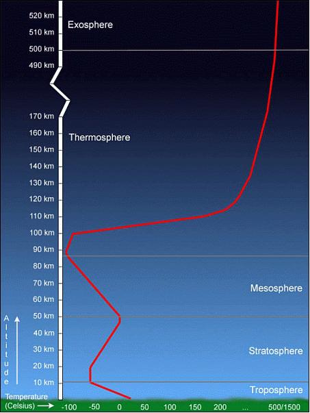
The Earth’s lower thermosphere is an important interface region between the neutral atmosphere and the “space weather” environment. The NSF-sponsored OPAL (Optical Profiling of the Atmospheric Limb) mission is designed to map global thermospheric temperature variability at mid- and low-latitudes over the critical “thermospheric gap” region (~100-140 km altitude) where prior data are sparse. Energy deposited into this region at high latitudes by geomagnetic storms is believed to be the most important driver of the global thermospheric temperature variability, but relatively little is known about the thermal response of the atmosphere as the energy is transported to mid- and low-latitudes. During the recent extended solar minimum period it became evident that large amounts of wave energy and momentum from the lower atmosphere are capable of penetrating well into the thermosphere, however little is known of the event signatures and regional impact. The goals of this mission are to further our understanding of the global thermospheric response to dynamic solar forcing and wave coupling from the lower atmosphere.
A-band temperature sensing: OPAL will profile the thermosphere temperature from
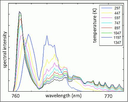
90 to 140 km altitude by observing the daytime O2 A-band emission using a high-sensitivity, compact, snapshot-hyperspectral limb imager. OPAL measures the thermosphere temperature by spectroscopic analysis of the molecular oxygen A-band emission (758 – 768 nm).
The emission lines that comprise the A-band (Figure 1) are grouped into two branches (R-branch below 662.1 nm, P-branch above). The shapes and relative strength of the two branches depend on the distribution of molecular rotation modes. Thus analysis of high resolution A-band spectra reveals the temperatures of the neutral atmosphere. Absolute radiometric calibration of emission intensities is not required.
The limb sensing instrument observes A-band spectra that combine emissions from the tangent radius upward. A sequence of spectra vs. elevation may be deconvolved to derive A-band spectra vs. altitude. These derived spectra are then fit to an A-band model to find the altitude profile of the neutral thermosphere temperature. This analysis process has been successfully applied to A-band data from the OSIRIS (Optical Spectrograph and Infrared Imaging System) instrument on the Odin mission and the NIRS (Near Infrared Spectrometer) instrument of RAIDS (Remote Atmospheric and Ionospheric Detection System), operated from the Kibo module of the ISS.
Spacecraft
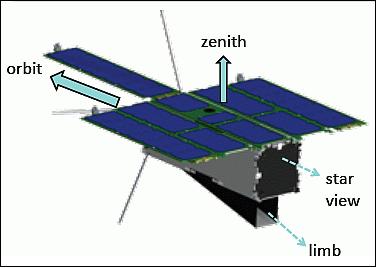
The OPAL spacecraft uses a Colony-II bus, provided by NRO (National Reconnaissance Office). The OPAL spacecraft is powered by six solar panels (one fixed, five deployed). A complete set of ADCS (Attitude Determination and Control Subsystem) instrumentation maintains a precise spacecraft orientation parallel to the velocity vector with the target limb scene directed aft (LVLH orientation) and LOS (Line of Sight) approximately 16° below the horizontal. Continuous limb observations will be provided during the day and in twilight.
The aft half of the spacecraft internal volume contains the bus electronics, including avionics, communication, battery, power, and data recorder. The forward half of the volume, 95 x 95 x 150 mm, is allocated to the limb-scanning spectrometer and other payload elements.
• The EPS (Electrical Power Subsystem) uses 6 solar panels
• ADCS: Use of an IMU (Inertial Measurement Unit) and 2 star trackers. Active attitude control with reaction wheels; ±0.25º stability. A star camera is used for enhanced LOS knowledge.
• RF communications: S-band radio (L3 Cadet radio of L3 Communication Systems).
The description of the spacecraft and its subsystems will be completed when available.
Launch
OPAL is expected to launch in late 2016 with a mission duration > 9 months. Most probably, OPAL will be launched on a resupply flight to the ISS.
Orbit: Near circular orbit, altitude of ~ 370 km, inclination = 51.6º.
Mission Status
- November 2020: The CubeSat bus that was initially supposed to host the OPAL instrument encountered problems during on-orbit tests, causing the bus development to be canceled. Nevertheless, the imaging instrument was fully developed and tested, and can now board other spacecraft if needed.7)
Sensor Complement
OPAL Instrument
The OPAL (the sensor and spacecraft have the same name) instrument is a high resolution imaging spectrometer that simultaneously collects spatially-resolved A-band spectra in multiple azimuthal directions and across the full altitude range of A-band emission. As the temperature increases, the relative intensity of the R branch (759 - 762 nm) increases and shifts to shorter wavelength while the P branch (762 - 770 nm) widens and shifts to longer wavelength. Thus, the neutral temperature (Tn) can be estimated from the qualitative shape of the A-band spectrum over the temperature range 150 - 1500 K (Ref. 3).
OPAL is a grating-based imaging spectrometer with refractive optics and a high-efficiency VHG (Volume Holographic Grating). The optical path is folded into three legs, each about 80 mm long. The scene is sampled by 7 parallel slits that form non-overlapping spectral profiles at the focal plane with a resolution of 0.5 nm (spectral), 1.5 km (limb profiling), and 60 km (horizontal sampling).
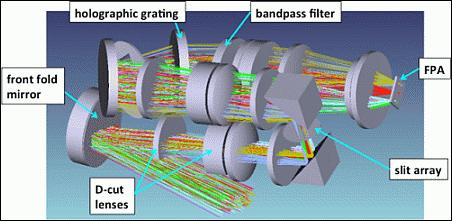
OPAL is a high-dispersion multi-slit imaging spectrometer. The functional design is illustrated in Figure 3. Light from the limb scene enters the instrument via a tilted front fold mirror that is coincident with a 5 x 14 mm rectangular entrance pupil. The scene is imaged onto the slit array by a 4-element lens assembly (group 1). The slits each sample a vertical limb profile with a horizontal sample spacing of 1.7º.
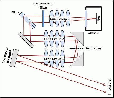
Light passing through the slits is recollimated by a second 4-element telecentric lens assembly (group 2) identical to the first. The light is dispersed along an axis perpendicular to the slits by a high-efficiency VHG aligned to the Littrow condition (incidence angle ~ diffraction angle). A narrow-band spectral filter blocks all wavelengths outside the A-band. A final four-element lens assembly (group 3) reimages the slits onto a FPA (Focal Plane Array).
The dispersion of the slit images is less than the spacing between the slit images. The FPA image thus consists of non-overlapping A-band spectra for each point on each slit. The spectral resolution (limited by the 49 µm slit width) is 0.5 nm. Because the OPAL instrument simultaneously collects high-resolution spectra that are resolved along two spatial dimensions, it is an example of a “Snapshot Hyperspectral” instrument. 6)
A CCD camera at the instrument focal plane delivers low noise and high sensitivity. The instrument is designed to strongly reject stray light from daylight regions of the Earth.
The OPAL spectrometer design illustrated in Figure 5 is entirely comprised of COTS (Commercial off-the-Shelf) components, except for the bandpass filter and VHG, which are inexpensive semi-custom elements. The first two elements of lens group 1 are cut down to avoid obstruction of the entrance aperture.
Folding of the optical path is addressing several considerations:
• The maximum package length is 150 mm, including the camera housing.
• The front fold mirror is approximately centered at the fore end next to the nadir surface to maximize the external shade length.
• Tolerances are provided for housings around each leg of the optical path.
• The FPA is positioned near the spacecraft centerline to leave room for the camera housing.
The folded configuration requires rotation of the slit array, VHG, and FPA to maintain orientation of the slit images and spectral dispersion with respect to the limb edge.
A preliminary design for the instrument mechanical packaging is illustrated in Figure 6 with a side panel removed. The top surface in the figure represents the nadir surface of the payload. Scene illumination enters through the slot in this surface.
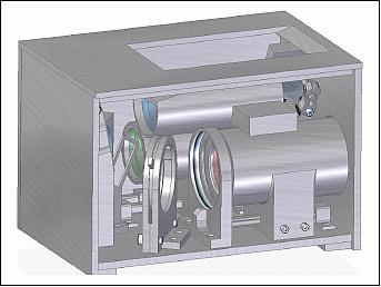
Each lens group is built as an assembly that is optically tested and aligned prior to instrument integration. Component coalignment is controlled by a unitary optical bench structure for mechanical and thermal stability. A subset of the component mounts provide fully-lockable adjustments for tip/tilt and azimuth rotation to control buildup of alignment errors through the complex optical path.
Camera and FPA: Image sensing for the OPAL spectrometer is performed by a commercial CCD camera, model Trius SX9 from Starlight Xpress, shown in Figure 7. The sensor is a Sony ICX285AL monochrome CCD (Figure 7, right) with 1392 x 1040 pixels at a 6.45 µm pitch. The photon detection efficiency in the A-band is 32%. The camera provides 16 bit readout over a USB interface with rms readout noise of only 5 e-. The ultra-low dark current (0.1 e-/s/pixel at 10ºC) supports the extended exposure necessary to observe the A-band emissions. The team confirmed the dark current and noise performance.
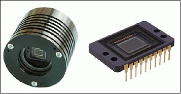
The Trius SX9 package is 70 mm long and 75 mm in diameter. The thermal fins on the housing will be machined back to fit the payload volume. The camera power is dominated by a TE cooler that stabilizes the sensor temperature. For OPAL, the set point (~10ºC) is close to ambient, minimizing the power and heat. Cooling is provided by an external radiator linked directly to the camera housing.
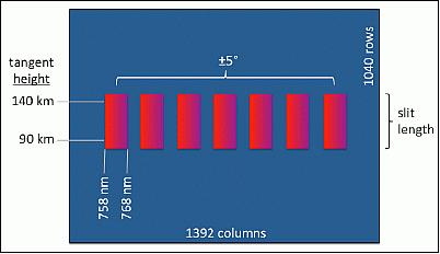
Utilization of the focal plane area is illustrated in Figure 8. The seven slits form discrete blocks of spectra spread in a band across the focal plane. Each block is a separate vertical profile across the limb covering a 10º horizontal FOV (Field of View). Each spectral block is 100 pixels wide corresponding to the nominal spectral band of 758 – 768 nm. The blocks are separated by gaps of 40 pixels that accommodate filter roll-off beyond the edges of the A-band. The height of each block is 240 pixels, including the vertical FOV plus an absolute pointing uncertainty of ±0.25º. Utilization of the focal plane for spectral data is less than 20%. Other regions of the focal plane may be utilized to monitor sensor offset and background stray light.
Concept of operations
The OPAL mission will take advantage of a launch into LEO (Low Earth Orbit). The architecture of the OPAL instrument can accommodate altitudes from 300 – 600 km. Because the most likely launch is an ISS resupply mission, the nominal OPAL orbit is 350 km with 51.6º inclination.
The typical daytime A-band brightness of the Earth limb ranges from 7,000 kR (kilo Rayleigh ) at 90 km tangent height to 100 kR at 140 km. With such a faint target, it is essential to maximize the exposure time. The nominal exposure time of 20 s corresponds to a longitudinal spatial resolution of 150 km (along the line of sight).
The Colony-II bus will maintain a fixed attitude with respect to the Earth, with the instrument FOV centered on the aft limb. Spectral images of the limb will be collected continuously, mapping out the thermosphere temperature profile in a swath surrounding the orbit. In the future, the project hopes to deploy a constellation of instruments spread out along a common orbit. Such a constellation could observe the rapid dynamic response of the thermosphere to energy input events.
Performance predictions
The net optical throughput of the instrument is estimated at 40%, including losses for the bandpass filter, VHG, and antireflection (AR) coated lenses, mirrors, and windows. Even with a 20 s exposure, the focal plane operates far below saturation with 2700 e-/pixel of accumulated signal at 90 km down to 38 e-/pixel at 140 km. At the bright lower edge, temporal noise is dominated by photon shot noise. At the top of the limb, shot noise and readout noise contribute about equally.
The nominal vertical and spectral resolution of OPAL are 5 km and 0.5 nm, respectively. Each resolution element corresponds to 14 x 5 pixels on the focal plane. Thus, the radiometric performance includes aggregation of signal and noise from 70 pixels.
The aggregate radiometric SNR (Signal to Noise Ratio) is predicted to range from 400 at the bottom of the limb to 40 at the top. Derivation of the temperature from the A-band spectrum includes a further combination of 20 samples per spectrum to fit a single temperature parameter. The rms temperature uncertainty estimated from analysis simulations ranges from 0.1K at the bottom of the limb to 13 K at 140 km. The 13 K uncertainty at the top of the limb represents a relative uncertainty of only 2%, because the thermosphere temperature there is typically > 600 K.
Stray light
OPAL will observe faint limb emissions under daylight conditions. Thus, control of stray light is a dominant consideration for the instrument design.
Internal surfaces
The optical path is fully enclosed from the entrance aperture to the camera, preventing cross-over of light between folded sections. The internal surfaces receive flat-black surface treatments, e.g. Z306 paint with diffuse reflectance Rdiff ~ 5%. To suppress ghosting, the lens surfaces are given narrow-band AR coatings with R<0.2% and the optical windows have broadband AR coatings with R < 2%.
For visually defect free optical surfaces, scattering is dominated by small angle “veiling glare” caused by microscopic surface roughness. All internal components are specified with 20Å rms roughness. The most critical optical surface (with by far the greatest stray light irradiance) is the front fold mirror. This is a superpolished dielectric mirror with rms roughness of 1 Å. The handling of this component during integration is critical.
Baffling
The instrument is designed to strongly reject stray light from daylight regions of the Earth that are as close as 2º below the limb scene. Sunlit clouds may be as bright as 106 kRad/nm, a thousand times brighter than the target at 90 km altitude. Straylight is restricted within the spectrometer by two pupil stops, the slit array, and the bandpass filter.
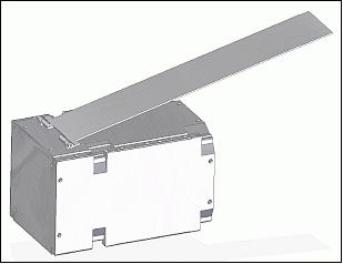
The narrow 5 mm height of the entrance pupil (positioned on the front fold mirror) facilitates external baffling within the size constraints of a CubeSat payload. An external shade assembly deployed from the nadir surface of the bus provides 250 mm of effective shade length, sufficient to prevent earthshine from directly or indirectly illuminating the entrance pupil.
Deployment of the spring-loaded bottom panel of the shade assembly is illustrated in Figure 9. As it is deployed, this panel also draws out flexible side walls (not shown) and an aft vertical panel that includes the baffle aperture (Ref. 3).
References
1) “National Scientific Foundation (NSF) CubeSat-based science missions for Geospace and Atmospheric Research,” Annual Report, October 2013, pp: 36-37, URL: http://www.nsf.gov/geo/ags/uars/cubesat/nsf-nasa-annual-report-cubesat-2013.pdf
2) “OPAL (Oxygen Photometry of the Atmospheric Limb)”, USU/SDL, URL: https://web.archive.org/web/20170614105524/http://www.sdl.usu.edu/downloads/opal.pdf
3) Alan Marchant, Mike Taylor, Charles Swenson, Ludger Scherlies, “Hyperspectral Limb Scanner for the OPAL Mission,” Proceedings of the AIAA/USU Conference on Small Satellites, Logan, Utah, USA, August 2-7, 2014, paper: SSC14-VII-5
4) Stephanie W. Sullivan, “Optical Sensors for Mapping Temperature and Winds in the Thermosphere from a CubeSat Platform,” Thesis for Master of Science in Electrical Engineering at USU, 2013, URL: http://digitalcommons.usu.edu/etd/1488/
5) Information provided by Alan Marchant of USU/SDL, Logan, UT, USA.
6) Nathan Hagen, Robert T. Kester, Liang Gao, Tomasz S. Tkaczyk, “Snapshot advantage: a review of the light collection improvement for parallel high-dimensional measurement systems,” Optical Engineering, Vol. 51, No. 11, June 13, 2012, URL: http://www.ncbi.nlm.nih.gov/pmc/articles/PMC3393130/
7) "Award Abstract # 1242901: CubeSat: The Optical Profiling of the Atmospheric Limb (OPAL) CubeSat Experiment", National Science Foundation (NSF), 25 November 2020, URL: https://www.nsf.gov/awardsearch/showAward?AWD_ID=1242901
The information compiled and edited in this article was provided by Herbert J. Kramer from his documentation of: ”Observation of the Earth and Its Environment: Survey of Missions and Sensors” (Springer Verlag) as well as many other sources after the publication of the 4th edition in 2002. - Comments and corrections to this article are always welcome for further updates (eoportal@symbios.space).
Overview Spacecraft Launch Sensor Complement References Back to Top