OCO (Orbiting Carbon Observatory)
EO
Atmosphere
NASA
Mission complete
Quick facts
Overview
| Mission type | EO |
| Agency | NASA |
| Mission status | Mission complete |
| Launch date | 24 Feb 2009 |
| End of life date | 24 Feb 2009 |
| Measurement domain | Atmosphere |
| Measurement category | Trace gases (excluding ozone) |
| Measurement detailed | CO2 Mole Fraction |
| Instruments | Spectrometer (OCO) |
| Instrument type | Atmospheric chemistry |
| CEOS EO Handbook | See OCO (Orbiting Carbon Observatory) summary |
OCO (Orbiting Carbon Observatory)
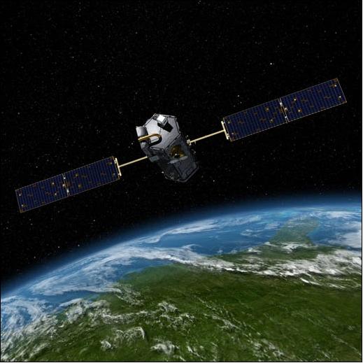
OCO is a NASA sponsored minisatellite mission selected in July 2002 within the ESSP (Earth System Science Pathfinder) program. The OCO science objective is to provide global measurements of atmospheric carbon dioxide (CO2) needed to describe the geographic distribution and variability of carbon dioxide sources and sinks. CO2 measurements are essential to resolving significant discrepancies in our understanding of the global carbon budget and, hence, humankind's role in global climate change. 1) 2) 3) 4) 5) 6) 7)
The Orbiting Carbon Observatory, a mission that partners with industry and academia, will generate knowledge needed to improve projections of future carbon dioxide levels within Earth's atmosphere. Increasing carbon dioxide (CO2) concentrations have raised concerns about global warming. Even though the biosphere and oceans are currently absorbing about half of the CO2 generated by human activities, the nature and geographic distribution of these CO2 sinks are too poorly understood to predict their response to future climate and land-use changes. The OCO mission is led and managed by JPL (PI: David Crisp). The project includes more than 19 universities as well as corporate and international partners (investigators from the USA, France, Germany, New Zealand, and Australia).
Spacecraft
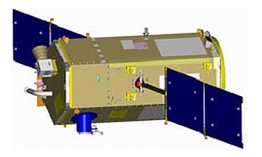
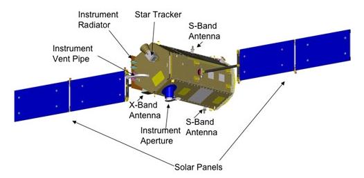
The OCO satellite is three-axis zero-momentum stabilized, using the LeoStar-2 bus of OSC [LeoStar-2 is of SORCE (Solar Radiation and Climate Experiment) and GALEX (Galaxy Evolution Explorer) heritage]. The platform is being used to point the instrument to nadir, glint, specific ground targets, or the limb, or to orient the calibration target toward the sun. It will also be used to point the body-mounted X-band antenna at the ground station twice each day. The estimated pointing accuracy is better than 900 arcsec, and pointing knowledge is better than 200 arcsec. The AOCS uses 4 reaction wheels as actuators to control the pitch, roll, and yaw of the bus. A set of 3 magnetic torque rods is used to de-spin the reaction wheels. Attitude is sensed by an IMU (Inertial Measurement Unit) and a star tracker. A GPS receiver provides location and timing data.
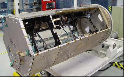
The spacecraft bus is a 2.12 m long hexagonal structure that is 0.94 m in diameter. Electrical power is provided by a pair of deployable solar panels that provide > 900 W when illuminated at near normal incidence. A pair of actuators is used to rotate these panels around the pitch (y) axis of the spacecraft bus to track the sun. The panels are used to charge a 35 Ahr nickel-hydrogen (NiH2) battery that provides power during eclipse. The spacecraft dry mass is ~315 kg, the wet mass is 460 kg. The mission design life is two years. 8) 9)
The hydrazine mono-propellant propulsion subsystem carries 45 kg of fuel to raise the orbit from the injection altitude (~635 km) to the operational orbit (705 km), adjust the orbit inclination as necessary, maintain the orbit during its 2-year nominal lifetime, and then de-orbit the Observatory at the end of the mission.
Launch
A launch of OCO took place on Feb. 24, 2009 on a Taurus-XL (3110) vehicle of OSC (Orbital Science Corporation) from VAFB, CA, USA.
Unfortunately, the OCO satellite failed to reach orbit. Preliminary indications are that the fairing on the Taurus XL launch vehicle failed to separate. The fairing is a clamshell structure that encapsulates the satellite as it travels through the atmosphere. NASA is convening a mishap investigation board to determine the cause of the launch failure. 10)
Orbit
Sun-synchronous orbit, altitude = 705 km, inclination = 98.2º, period = 98.8 min, repeat cycle of 16 days, equatorial crossing time at 13:15 hours on an ascending node. The OCO S/C will become part of the “A-Train” (a loose formation of the Afternoon Constellation consisting of: Aqua, CloudSat, CALIPSO, PARASOL, Aura, and OCO) to correlate the OCO data with data acquired by other instruments such as AIRS on Aqua. OCO will fly ahead of the A-train, about 15 minutes before the Aqua spacecraft.
The OCO flies at the head of the A-Train, 12 minutes ahead of the Aqua platform.
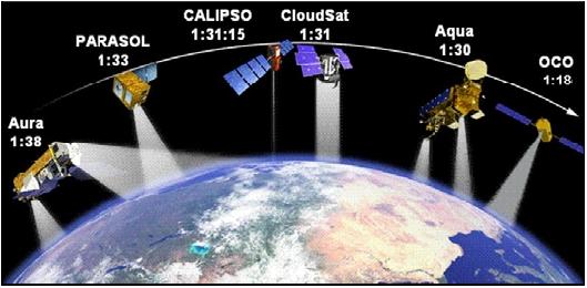
Note: The observatory will initially be launched into a 640±30 km transfer orbit. Once the spacecraft bus has been checked out, the orbit will be raised to 705 km altitude, to fly in formation with the Earth Observing System (EOS) Afternoon Constellation (A-Train).
RF Communications
Onboard data storage volume of 128 Gbit. The science data downlink is in X-band at a data rate of 150 Mbit/s. In addition, an S-band link is provided for TT&C operations (max. downlink rate at 2 Mbit/s). The TT&C link can also be routed via TDRSS. Spacecraft monitoring will be performed at OSC, Dulles, VA. Science data acquisition, archiving, processing and distribution is being done at JPL.
Sensor Complement (OCO Instrument)
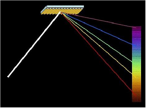
Measurement approach of the OCO instrument: The OCO spacecraft carries a single instrument that incorporates three high-resolution and co-aligned grating spectrometers to measure reflected sunlight off the Earth's surface in the 0.76 µm O2 A-band, and the CO2 bands at 1.61 and 2.06 µm. A simultaneous retrieval algorithm will be used to retrieve time-dependent estimates of the column-averaged CO2 dry air mole fraction, XCO2. The OCO mission incorporates a comprehensive ground-based validation and correlative measurement program to ensure the accuracy of the space-based XCO2 measurements have precisions of 0.3% (1 ppm CO2) on regional scales. Once validated, the space-based XCO2 measurements will be combined with groundbased and aircraft measurements and incorporated into sophisticated source-sink inversion and data assimilation models to characterize the geographic distribution of CO2 sources and sinks over two annual cycles.
The spectral range of each channel includes the complete molecular absorption band as well as some nearby continuum to minimize biases due to uncertainties in atmospheric temperature and to provide constraints on the optical properties of the surface albedo and aerosols. The spectral resolving power for each channel was selected to maximize the sensitivity to variations in the column abundances of CO2 and O2, and to minimize the impact of systematic measurement errors. A spectral resolving power, lambda/delta lambda ~21,000 separates individual CO2 lines in the 1.61 and 2.06 µm regions from weak H2O and CH4 lines and from the underlying continuum. For the O2 A-band, a resolving power of ~17,000 is needed to distinguish the O2 doublets from the continuum. With these resolving powers, the OCO retrieval algorithm can characterize the surface albedo throughout the band and solve for the wavelength dependence of the aerosol scattering, minimizing XCO2 retrieval errors contributed by uncertainties in the continuum level.
The OCO instrument is being designed and developed by HSSS (Hamilton Sundstand Sensor Systems), Pomona, CA, the manufacturer of the last four TOMS instruments (the parent company of HSSS is United Technologies Corporation). 11) 12) 13) 14)
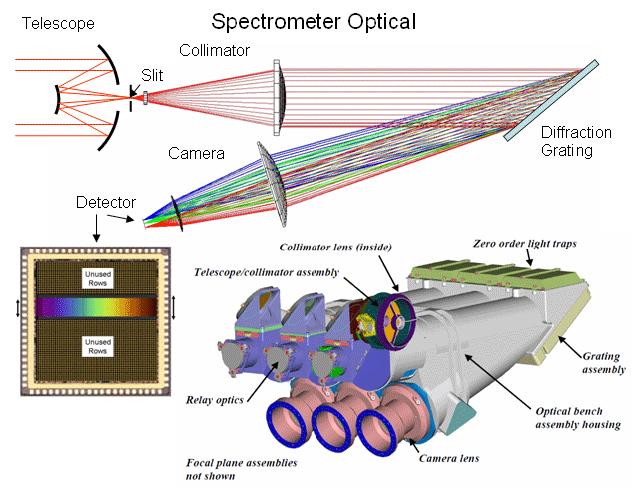
The OCO instrument package incorporates independent bore-sighted, longslit, imaging grating spectrometers for observations in the 1.61 µm and 2.06 µm CO2 bands and the 0.76 µm O2 A-band. A single telescope is coupled to the entrance slits of the three grating spectrometers using a dichroic relay system to ensure the spectrometers share the same field of view. An unusual all reflective-transmission diffuser provides for on orbit spectral/radiometric solar calibration. Behind the slit, the light is collimated, dispersed by a grating, and focused by a camera lens, forming an image of a spectrum on a FPA (Focal Plane Array). The spectrum is dispersed across the FPA in the direction orthogonal to the slit, and (cross-track) spatial information is recorded along the slit.
| 0.76 µm O2 | 1.61 µm CO2 | 2.06 µm CO2 | |||
Requirement | Specification | Prediction | Specification | Prediction | Specification | Prediction |
FOV (mrad) | ≤ 1.9 | 1.8 | ≤ 1.9 | 1.8 | ≤ 1.9 | 1.8 |
Samples | 14.2 - 15.1 | 14.6 | 14.2 - 15.1 | 14.6 | 14.2 - 15.1 | 14.6 |
Pixels/sample | 8 | 8 | 8 | 8 | 8 | 8 |
Min wavelength (µm) | ≥ 19 | 20 | ≥ 19 | 20 | ≥ 19 | 20 |
Max wavelength (µm) | 0.772 | 0.772 | 1.621 | 1.621 | 2.081 | 2.081 |
Spectral resolution | ≥17,000 | 17,842 - 18,199 | ≥ 20,000 | 20,990 - 21,410 | ≥ 20,000 | 20,990 - 21,410 |
Spectral sampling pixels/sample | ≥ 2 | 2.45 - 3.34 | ≥ 2 | 2.08 - 2.84 | ≥ 2 | 2.08 - 2.84 |
Optical sampling TM(s) polarization | > 35% | 35.5% | > 40% | 41.5% | > 45% | 46.3% |
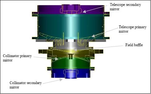
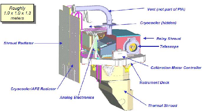
The spectrometers are illuminated by a common 110 mm diameter aperture Cassegrain telescope. The light is transmitted through a set of relay optics to illuminate the 3 spectrometer slits. The relay optics assembly includes a collimating mirror, fold mirrors, dichroic beam splitters, band isolation filters and re-imaging mirrors. Each spectrometer consists of a slit, a two-lens collimator, a grating, and a two-lens camera. The focal ratios of the instrument optics range from f/1.6 to f/1.9.
The OCO instrument design combines refractive and reflective optical techniques to achieve a fast and effective measurement system. The stacked array of apertures, shaped mirrors and reflective diffusers allows the irradiance profile filling the telescope entrance pupil to be tailored to perform solar calibration of the OCO spectrometers over their full dynamic range when in this mode and the instrument is oriented to view the sun directly. This proved impossible to achieve using traditional reflective or transmission diffuser designs. All surfaces in the all-reflective transmission diffuser are coated with gold.
To obtain enough useful soundings to accurately characterize the XCO2 distribution on regional scales, even in the presence of patchy clouds, the OCO instrument continuously records 4 soundings along a 0.4º wide cross-track swath at 3 Hz, yielding 12 soundings/s. As the spacecraft moves along its ground track at about 6.78 km/s, each sounding exhibits a surface footprint with dimensions of ~1.29 km x 2.25 km at nadir. About 196 soundings are recorded over each 1º latitude increment along the orbital track.
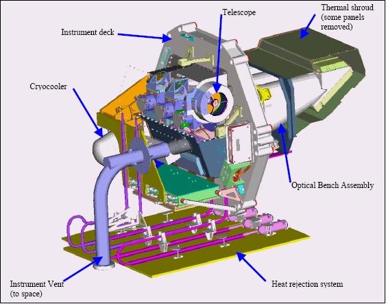
The 3 spectrometers are integrated into a common structure (optical bench assembly) to improve rigidity and thermal stability. Behind the slit, the light is collimated, dispersed by a grating, and focused by a camera lens, forming a two-dimensional image of a spectrum on a 1024 x 1024 pixel focal plane array (FPA). OCO employs all 1024 of the pixels in the spectral dimension but only 220 of the pixels in the spatial dimension. The FPAs are being cooled by a pulse tube cryocooler of NGST (Northrop Grumman Space Technologies, formerly TRW) to 120 K for the 2.06 µm band and 220 K for the 0.76 µm band. Note: The cryocooler is actually the flight spare of the TES (Tropospheric Emission Spectrometer) instrument, flown on NASA's Aura mission with a launch July 15, 2004.
The spectrum is dispersed across the FPA in the direction orthogonal to the slit, and spatial information is recorded along the length of the slit. The slit length defines a 10 km wide cross-track swath at nadir from a 705 km orbit. This cross-track FOV is resolved by 160 pixels (16% of the array). These cross-track pixels are summed into 16 pixel bins to produce ten independent cross-track samples.
The slit width defines an IFOV (Instantaneous Field of View) of ~0.1 mrad.. From a 705 km orbit, this corresponds to an along-track range of ~750 m. When the spacecraft is flying with it z axis aligned with the orbit track, this IFOV convolves with the spacecraft motion to yield the 2.25 km along-track footprint at nadir (3 Hz samples). The cross-track IFOV is also < 0.1 mrad, but cross-track elements are summed onboard to reduce the downlink data volume. This approach produces the 1.29 km cross-track field at nadir.
Parameter | Value | Parameter | Value |
Instrument type | 3 high-resolution grating spectrometers | Sampling modes | Nadir, Glint, Target |
Min wavelength | O2 A-band: 0.758 µm | Max wavelength | O2 A-band: 0.772 µm |
Resolving power (lambda/delta lambda) | O2 A-band: > 17,000 | Spatial resolution | 1.29 km (cross-track x 2.25 km (along-track) |
FOV (swath) | 14 mrad in cross-track | IFOV (pixel) | 0.09 mrad (along-track) |
Instrument mass, power | ~ 150 kg, < 165 W | Instrument size | 1.6 m x 0.4 m x 0.6 m |
Temperature of optics | 268-273 K | Temperature of detectors | 120-189 K |
Duty cycle | On continuously, but science data are recorded only over the sunlit hemisphere | Source data rate | ~ 1 Mbit/s |
Measurement accuracy | Single sounding XCO2 accuracy of better than 2%, regional scale XCO2 accuracy of 0.3% on monthly time scales | ||
Calibration | - Absolute radiometric: Diffuse solar spectrum transmitted through entire optical system. | ||
Product name or group | Processing level | Coverage | Spatial/temporal parameters |
Calibrated radiance-spectra of O2 A-band 1.61 and 2.06 µm CO2 bands | 1 B | Atmospheric column | 1.29 km x 2.25 km horizontal resolution, 16 days |
Column-averaged dry air mole fraction, XCO2 | 2 | Atmospheric column | 1.29 km x 2.25 km horizontal resolution, 16 days |
Regional-scale XCO2 | 3 | Atmospheric column | 103 km x 103 km horizontal resolution, monthly |
Sources and sinks | 4 | Atmospheric column | 103 km x 103 km horizontal resolution, monthly |
Instrument Calibration
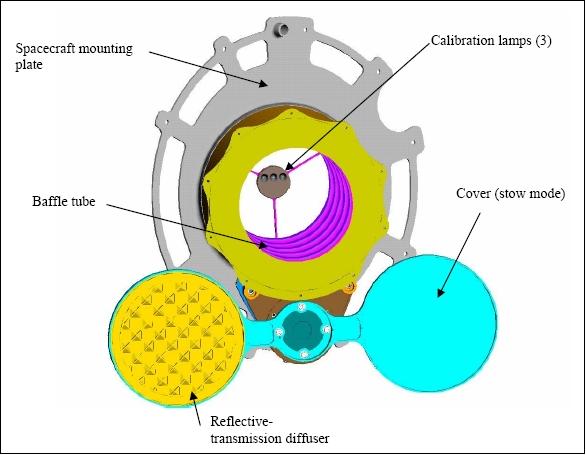
An on-board calibrator is integrated into the telescope baffle assembly (Figures 10, 11). An actuator rotates a “propeller” that carries an aperture cover (lens cap) and a transmission diffuser. The cover is closed to protect the instrument aperture during launch and orbit maintenance activities. The cover is also closed to acquire “dark frames” that are used to monitor the zero-level offset of the FPAs.
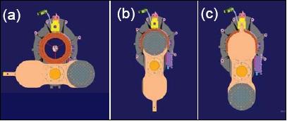
The inside of the cover has a diffusively reflecting gold surface that can be illuminated by one of 3 tungsten lamps installed the baffle assembly. These lamps are used to take “flat field” images that are used to monitor the relative gain of the individual pixels on the FPAs. The propeller is rotated 180º from the closed position to place the transmission diffuser in front of the telescope aperture to view the sun. Measurements of direct sunlight through the diffuser provide an absolute radiometric calibration of the instrument and yield solar spectra for the full range of Doppler shifts (± ~7 km/s) observed over the illuminated hemisphere. The propeller is rotated 90 degrees from either the closed or diffuser positions for normal science observations.
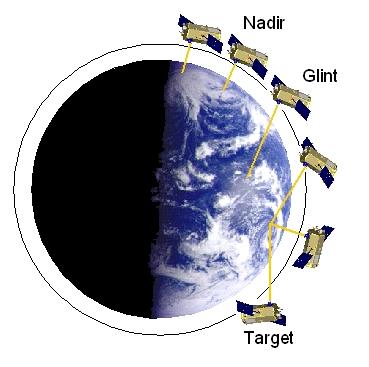
Observation Modes
To provide the mission with additional flexibility, the Observatory will acquire data in three different measurement modes. The following observation modes are provided (the same sampling rate of 12 soundings/s is used in each mode):
• Nadir mode: the instrument views the ground directly below the spacecraft (local nadir). Observations are made whenever the solar zenith angle is < 85º.
• Glint mode: the instrument views the location where sunlight is directly reflected on the Earth's surface (the OCO is pointed towards the bright spot where solar radiation is specularly reflected from the surface). The glint mode enhances the instrument's ability to acquire highly accurate measurements, particularly over the ocean. In particular, the Glint measurements over the ocean should provide much higher SNR values. Glint soundings are being collected at all latitudes - whenever the local solar zenith angle is < 75º. OCO switches from Nadir to Glint modes on alternate 16-day global ground-track repeat cycles so that the entire Earth is mapped in each mode on roughly monthly time scales.
• Target mode: the instrument views a specified surface target (calibration site) continuously as the satellite passes overhead (max pass duration up to 9 minutes). The Target mode provides the capability to collect a large number of measurements over sites where alternative ground-based and airborne instruments also measure atmospheric CO2.
Naturally, the size of the footprint increases when observations are made in Glint or in Target modes (that are different from nadir).
OCO provides near global coverage at monthly intervals to make space-based measurements of atmospheric carbon dioxide with the precision, resolution, and coverage needed to characterize the geographic distribution of CO2 sources and sinks and to quantify CO2 variability over the annual cycle.
OCO cycles between nadir and glint modes on 16-day intervals to cross calibrate observations. In the nadir mode, the instrument will collect footprints directly beneath the spacecraft with an area of less than 3 km2. The glint mode observes the solar radiance reflected specularly from the Earth's surface to improve the signal to noise ratio from the low albedo of the water's surface in these measurements bands. A 10.3 km wide swath at nadir is measured from a nominal orbit height of 705 km. The swath includes 8 cross-track samples of 20 pixels per sample. A rolling readout is incorporated resulting in parallelogram-shaped ground footprints.
Ground Truth
NASA/LaRC developed a ground-based DIAL (Differential Absorption Lidar) instrument with the capability to measure range-resolved and column amounts of atmospheric CO2. This system is also capable of providing high-resolution aerosol profiles and cloud distributions. The instrument is being developed as part of the NASA Earth Science Technology Office's IIP (Instrument Incubator Program). It will be a valuable tool in the validation of the OCO mission measurements of column CO2 and suitable for deployment in the NACP (North American Carbon Program) regional intensive field campaigns. 15)
The double-pulsed DIAL instrument features a 2.05 µm laser technology. The receiver uses an f/2.2 all aluminum 40 cm diameter telescope and the system is designed to focus light onto a 200 µm size detector. It uses a newly developed low noise and high gain InGaAsSb/AlGaAsSb (AstroPower) infrared heterojunction phototransistor (HPT) with a 200 µm sensitive area diameter. The receiver system employs two receiver channels to capture the full dynamic range of signals in the near (within the boundary layer 0.5 to 2.0 km range) and far field (above the boundary layer >1 km).
The system capabilities include measuring range-resolved and column amounts of CO2 with high-resolution, while profiling aerosol and cloud distributions. A high pulse energy, tunable, wavelength stabilized, and double-pulsed 2 µm laser is used as the transmitter. The laser is operable over preselected temperature insensitive strong CO2 absorption lines. An all-aluminum Cassegrain telescope is used in the receiver. Accompanied with state-of-the-art electronics and digitizer, system fine-tuning and testing is in progress.
References
1) D. Crisp, R. M. Atlas, F.-M. Breon, L. R. Brown, J. P. Burrows, P. Ciais, B. J. Connor , S. C. Doney, I. Y. Fung, D. J. Jacob, E. C. Miller, D. O'Brien, S. Pawson, J. T. Randerson, P. Rayner , R. J. Salawitch, S. P. Sander, B. Sen, G. L. Stephens, P. P. Tans, G. C. Toon, P. O. Wennberg, S. C. Wofsy, Y. L. Yung, Z. Kuang, B. Chudasama, G. Sprague, B. Weiss, R. Pollock, D. Kenyon, S. Schroll, “The Orbiting Carbon Observatory (OCO) mission,” Advances in Space Research, Vol. 34, 2004, pp. 700-709, URL: http://www.people.fas.harvard.edu/~kuang/OCO_mission.pdf
2) D. Crisp, C. Johnson, “The Orbiting Carbon Observatory Mission,” 4th IAA Symposium on Small Satellites for Earth Observation, Berlin, Germany, April 7-11, 2003
3) D. Crisp, C. Johnson, “The Orbiting Carbon Observatory Mission,” Acta Astronautica, Vol. 56 (1-2), Jan. 2005, pp. 193-197
4) Information provided by David Crisp of NASA/JPL, Pasadena, CA
5) David Crisp and the OCO Science Team, “Monitoring CO2 Sources and Sinks from Space: The Orbiting Carbon Observatory (OCO) Mission,” URL: [web source no longer available]
6) David Crisp, “The Orbiting Carbon Observatory: Sampling Approach and Anticipated Data Products,” Carbon Fusion Workshop, May 9-11, 2006, Edinburgh, Scotland, URL: http://www.geos.ed.ac.uk/carbonfusion/events/Crisp_OCO_Carbon_Fusion_2006.ppt
7) T. R. Livermore, D. Crisp, “The NASA Orbiting Carbon Observatory Mission,” Proceedings of the 2008 IEEE Aerospace Conference, Big Sky, MT, USA, March 1-8, 2008
8) “OCO Orbiting Carbon Observatory,” Orbital, URL: [web source no longer available]
9) "Orbiting Carbon Observatory," Orbital, URL: [web source no longer available]
10) “Overview of the Orbiting Carbon Observatory (OCO) Mishap Investigation Results For Public Release,” NASA, URL: http://www.nasa.gov/pdf/369037main_OCOexecutivesummary_71609.pdf
11) R. Haring, R. Pollock, B. Sutin, D. Crisp, “The Current Development Status of the Orbiting Carbon Observatory (OCO) Instrument Optical Design,” URL: [web source no longer available]
12) R. E. Haring, R. Pollock, B. M. Sutin, D. Crisp, “Development status of the Orbiting Carbon Observatory instrument optical design,” Optics & Photonics 2005, SPIE, San Diego, CA, USA, July 31-Aug. 4, 2005, SPIE Vol. 5883
13) Vijay Natraj, “The Orbiting Carbon Observatory (OCO) Mission,” March 1, 2006, URL: http://www.gps.caltech.edu/~vijay/Ge152/OCO%20Misson%20-%20Ge152.ppt
14) David Crisp, “The Orbiting Carbon Observatory: Sampling Approach and Anticipated Data Products,” May, 2006, URL: [web source no longer available]
15) S. Ismail, G. Koch, N. Abedin, T. Refaat, M. Rubio, U. Singh, “Development of Laser, Detector, and Receiver Systems for an Atmospheric CO2 Lidar Profiling System,” Proceedings of the 2008 IEEE Aerospace Conference, Big Sky, MT, USA, March 1-8, 2008