MSX (Midcourse Space Experiment)
EO
Multi-band UV/VIS Spectrometer (ACE)
Atmosphere
Multi-purpose imagery (ocean)
Quick facts
Overview
| Mission type | EO |
| Agency | DoD (USA) |
| Mission status | Mission complete |
| Launch date | 24 Apr 1996 |
| End of life date | 01 Jul 2008 |
| Measurement domain | Atmosphere, Gravity and Magnetic Fields |
| Measurement category | Multi-purpose imagery (ocean), Gravity, Magnetic and Geodynamic measurements, Atmospheric Humidity Fields, Lightning Detection |
| Instruments | Multi-band UV/VIS Spectrometer (ACE), TDP, HF Beacon Transmitter |
| Instrument type | High resolution optical imagers, Magnetic field, Other, Communications, Data collection, Lightning sensors |
| CEOS EO Handbook | See MSX (Midcourse Space Experiment) summary |
MSX (Midcourse Space Experiment)
Overview Spacecraft Launch Mission Status Sensor Complement MSX Ground Segment References
The MSX satellite is an observatory-class observation platform and global surveillance system of the US DoD; it is funded and managed by BMDO (Ballistic Missile Defense Organization) with JHU/APL (Johns Hopkins University/Applied Physics Laboratory) of Laurel, MD as the prime contractor, spacecraft integrator, and operator of the mission. MSX represents the first system demonstration in space of technology to identify and track ballistic missiles during their midcourse flight phase. The suite of optical sensors cover the spectrum from the far ultraviolet (110 nm) through the very-long-wave infrared (28 µm) spectrum. 1)
The primary objectives of MSX are to detect, acquire and track targets and to discriminate lethal from nonlethal objects (detailed characterization and modeling of target objects and their associated phenomenology of the terrestrial, Earth-limb, and celestial backgrounds). The information gathered by the MSX spacecraft will help fill significant spatial, spectral, and temporal gaps that currently exist in space environment models. Another driving factor in the MSX Program is sensor and spacecraft technology improvement. The latest technology is used to provide the most up-to-date phenomenological information and to serve as a new-technology demonstrator. 2) 3) 4) 5) 6)
In addition to meeting the needs of the BMDO, the MSX spacecraft provides a civilian benefit owing to its multispectral and hyperspectral capabilities. Data collected from BMDO-related experiments can be used to perform environmental studies of the Earth. Special environmental monitoring experiments can also be conceived and performed.
The initial architecture concept for the SDI (Strategic Defense Initiative) was a multi-phased approach. A series of highly sensitive surveillance and weapons control sensor systems which had to provide robust discrimination capabilities were key to the first phase. The MSX (Midcourse Space Experiment) was conceived as a an early demonstration of critical technologies and functions for midcourse sensors. MSX supported SDI objectives by providing the system functional demonstrations, target and background data, and the technology demonstrations necessary for the midcourse sensor platforms. The primary mission of the MSX was to demonstrate the ability to acquire and track realistic midcourse objects against realistic backgrounds. Target experiments employed system-representative ranges, geometries, resolutions, and frame rates, and used existing IR technology with legacy to future operational sensors. As a space demonstration for the Strategic Defense Initiative Organization midcourse sensor concepts, MSX gathered data and explored limits to which midcourse functions could be performed. These functions included acquisition, cluster track, and resolution, bulk filtering, discrimination, handover, and multi-sensor fusion. 7)

Spacecraft
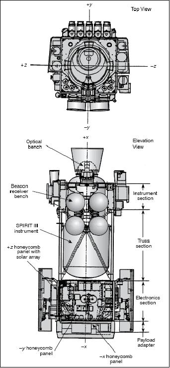
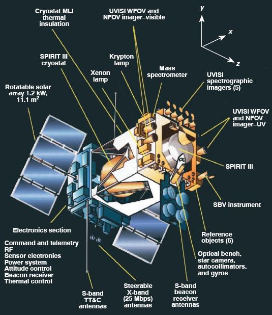
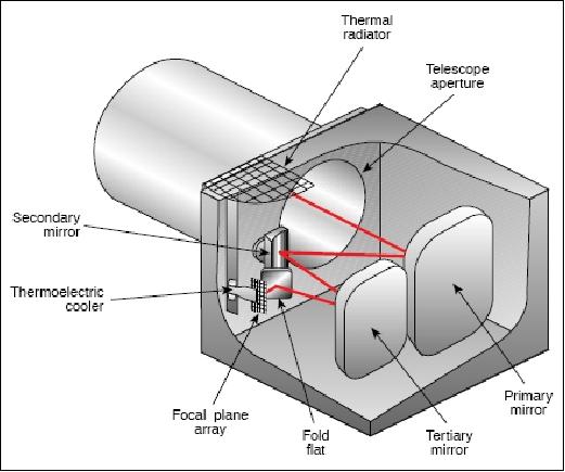
The MSX satellite is three-axis stabilized consisting of the structure, five primary instrument systems, and the subsystems needed for instrument support and S/C control. The fundamental configuration was required by the size and thermal requirements of SPIRIT-III (Spatial Infrared Imaging Telescope-III). The spacecraft structure is divided into three discrete elements consisting of (Figure 2): 8) 9)
1) An electronics section, which provides an interface to the Delta II launch vehicle and a mounting platform for instrument and spacecraft electronics.
2) Truss section: A thermally stable graphite/epoxy composite truss structure for mounting the SPIRIT-III instrument and providing an interface between the instrument and electronics sections. A major design driver for the thermal team was to keep the average temperature of the SPIRIT-III outside shell below 250 K, with a goal of 225 K.
3) Instrument section: A temperature-controlled instrument section with embedded heat pipes for mounting delicate sensors and instruments. The instrument section also provides a thermally stable mounting structure for the optical bench and the beacon receiver bench.
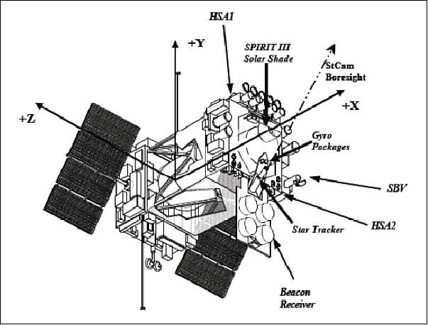
The instrument section also contains two ancillary structures that play an important role in the tracking and attitude control of the spacecraft. The optical bench is a precision inertial measurement platform that is attached to the top of the instrument section structure. The G/E (Graphite/Epoxy) composite bench supports the ring laser gyroscopes and a star camera for establishing and maintaining spacecraft attitude control. The G/E composite bench contains four S-band receiving antennas that can acquire and lock onto a target signal beacon at frequencies of 2219.5 and 2229.5 MHz during spacecraft tracking activities.
The instrument section is a four-sided box structure that provides mounting locations for most of the spacecraft sensors. The entire section is blanketed. It contains the SBV instrument telescope, the UVISI instruments, and the contamination experiments. The section is cut away in the middle to allow for the SPIRIT-III telescope.
The MSX spacecraft has a design life of five years, its body measures approximately 160 cm x 160 cm x 520 cm, and its launch mass is about 2812 kg.
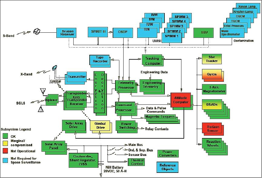
The ADCS (Attitude Determination and Control Subsystem) consists of four reaction wheels and three magnetic torque rods. Any three of the four wheels can provide three-axis control of the satellite. Attitude sensors include two three-axis ring laser gyro systems, a star camera, two horizon sensors, five digital sun-angle detectors, and a three-axis magnetometer. The system achieves a real-time pointing accuracy of better than 0.1º and post-processing knowledge of 9 µrad over instrument integration durations of about 1s.
Coarse attitude sensors | - MAG - a 3-axis magnetometer measured the Earth's magnetic filed |
Fine attitude sensors | - ST (Star tracker); measured up to five stars |
Rate sensors | - RLG (2x) - IRUs (Inertial Reference Units), ring-laser gyroscopes |
Actuation | - RWA (Reaction Wheel Assembly) with 4 wheels |
AP (Attitude Processors) | - Dual 1750 computers (2 x) |
Tracking processors | - 1750 computer (2 x) - all scenario calculations |
Modes | - Park & Track - coarse or fine attitude knowledge or propagated RLG data |
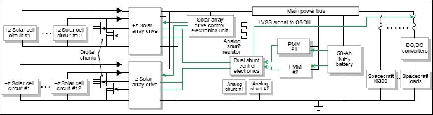
EPS (Electric Power Subsystem): An unregulated direct energy transfer topology of 28 VDC.. The solar array (1.2 kW BOL) consists of two wings, each comprising four solar panels supported by a boom and attached to a SAD (Solar Array Drive). The battery consists of a series stack of 22 rechargeable nickel-hydrogen (NiH2) cells with a capacity of 50 Ah. Redundant power management modules (PMMs), which monitor the battery and provide the main EPS command and data handling (C&DH) subsystem interfaces; and the dual shunt control electronics (DSCE), which control the analog and digital shunts and contain the low voltage sense system (LVSS) circuitry. 10)
C&DHS (Command and Data Handling Subsystem): The command subsystem consists of command processor, data handling, key generator (KG)/ tempest, power switching, and tape recorder components. Commands transmitted from ground stations are acquired via the S-band transponders.
Spacecraft science and housekeeping data are gathered by the DHS and formatted to generate three serial data outputs. Each stream has selectable formats and can be turned on and off independently as required by the mission. These three streams are the following: 11)
1) 25 Mbit/s (or 5 Mbit/s) prime science data stream containing imager, processor, and housekeeping data; transmitted in real time or stored on one of the spacecraft tape recorders
2) 1 Mbit/s snapshot science and housekeeping wideband downlink data stream; transmitted in real time
3) 16 kbit/s narrowband downlink data stream containing spacecraft housekeeping and memory dump data; transmitted in real time.
The C&DHS subsystem includes data encryption and decryption units and two tape recorders of Odetics, each with a storage capacity of 54 Gbit.
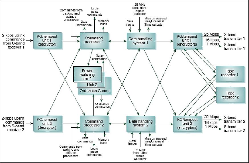
Figure 6: Functional block diagram of the C&DHS (image credit: JHU/APL)
Tracking Function of Targets
The target tracking experiments represent the primary mission of the MSX; they are in fact the main driver of spacecraft design. These experiments last about 30 minutes, with all sensors powered and collecting data and the spacecraft slewing at high rates to follow ballistic missile targets. 12)
The tracking experiments sized the spacecraft power, attitude, and data handling systems. There is also a tracking requirement which called for the capability of the spacecraft of performing a full target tracking experiment without solar input, to permit experiments to be done in eclipse phase of the orbit or with the solar panels in an unfavorable solar attitude position. Hence, a 50 Ah NiH2 battery was chosen to supply the needed power for such a target tracking event.
The MSX incorporates another function not normally seen in spacecraft: closed loop tracking on targets other than stars. As seen in Figure 3, a TP (Tracking Processor) can take sensor information from several sensors to acquire and closed-loop-track a target. These sensors are identified in the following list:
• Beacon receiver. This S-band passive radar tracker tracks telemetry transmitters on target vehicles. It has a much wider FOV (Field of View) than the optical instruments, and it guides spacecraft attitude, through the TP and attitude system, to point the target to well within the smaller field of view of the optical sensors.
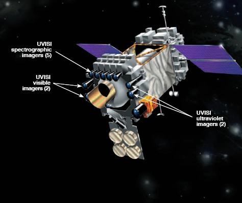
• UVISI (Ultraviolet and Visible Imagers and Spectrographic Imagers) narrow FOV visible imager, a 1.3º x 1.6º visible band imager.
• UVISI narrow FOV ultraviolet imager, a 1.3º x 1.6º ultraviolet imager.
• UVISI wide FOV visible imager, a 10.5º x 13.1º visible band imager.
• UVISI wide FOV ultraviolet imager, a 10.5º x 13.1º ultraviolet imager.
• SPIRIT-III radiometer. Band A or D can route images to an experimental target processor called the Onboard Signal and Data Processor, which routes target tracking information to the spacecraft TP.
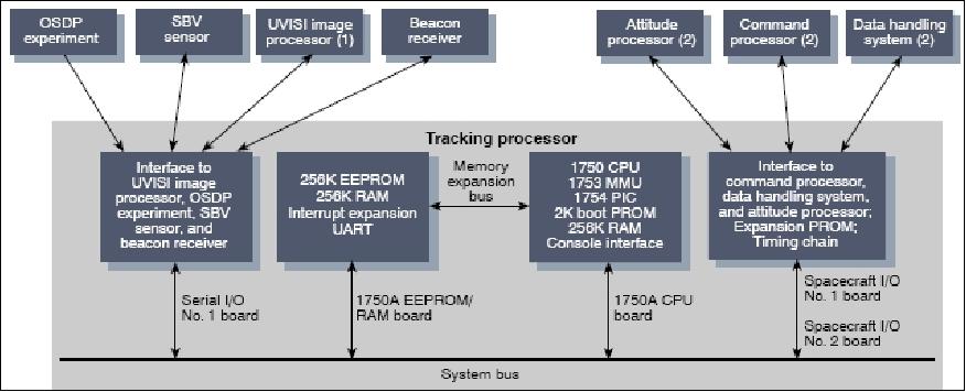
Figure 7: Block diagram of the tracking processor and interfaces (image credit: JHU/APL)
RF Communications
The MSX communicates on three bands: S-band uplink (1827.8 MHz), S-band downlink (2282.5 MHz), and X-band (8475 MHz). The S-band uplink is used exclusively for commanding and memory loads (data encryption). The S-band has two transponders, diplexers, and antenna pairs for the transmission of 16 kbit/s housekeeping data and either ranging or 1 Mbit/s transmission of compressed or sampled science data.
The X-band (two transmitters) transmits 25 (or 5) Mbit/s prime science data from the S/C data recorders (54 Gbit capacity each).
Beacon receiver antenna bench: This device is a 0.4 m2 panel that houses a four-parabolic-dish, phased-array antenna. It is folded down to stow against the side of the instrument section during launch and is released and pinned in place so its antenna beams are pointed in the same direction as the optical instruments. The S-band beacon receiver is a passive radar tracker that can acquire a target with an initial pointing uncertainty of ±5º at a maximum range of 8000 km. It provides calibrated angle tracking with a residual error of 0.1º.
Launch
The MSX spacecraft was launched on April 24, 1996 with a Delta-2 7920 vehicle from VAFB (Vandenberg Air Force Base), CA, USA.
Orbit
Near sun-synchronous polar orbit, altitude = 897 km x 907 km, inclination = 99.4º. The daily precession rate is < 0.04º.
This orbit allows the spacecraft to fly in a roughly Earth-oriented attitude while keeping direct sunlight out of the instrument apertures. Controlling the spacecraft's attitude relative to the sun is one requirement that shapes the whole mission.
Mission Status
• In July 2008, after more than 12 years of successful operations and contributions to two diverse defense missions, the MSX spacecraft was retired, having operated well beyond its design life of 4 years. The spacecraft collected vital data for designing missile defense systems. With no fuel onboard, reentry of the spacecraft will take place in a few centuries. 13) 14)
Decommissioning the MSX spacecraft did not consist of a series of deorbit maneuvers, as is the practice for some satellites, because it had no propellant. Nor was it as simple as just powering down the spacecraft components and walking away because the design of the spacecraft included a level of autonomous survival methods that were hard-coded into the flight software. Any decommissioning plan needed to account for the flight software design and to defeat those survival actions. 15)
The decommissioning goal was to place MSX in a state such that it would not generate any RF signature and would minimize any chances of debris. Because there was no propellant or other expendables on the spacecraft, the decommissioning planning revolved around depleting the MSX power subsystem to a level at which there would be insufficient energy to support any subsystem operation and insufficient energy for the spacecraft to autonomously reconfigure itself for survival.
The decommissioning of MSX marked the end of one of the most successful satellite programs ever undertaken by APL. The MSX spacecraft had fulfilled not only an ambitious primary mission, but it had also provided an abundance of useful data for a time well beyond its designed lifetime. The 12 years of active operations that followed years of development and testing at APL were filled with frequent adaptation to changing spacecraft capabilities as well as to sponsor needs. These changes presented challenges to the operations teams throughout the program, including during the decommissioning process (Ref. 15).
The objectives of the primary mission (of 1 year duration ) were: 16)
- Track ballistic missile targets to study phenomenology
- Survey horizon "clutter"
- Track rocket & missile launches
- Infrared star survey for calibration & cataloging
- Sensor performance evaluation
During the program's primary mission, the first year in orbit, it was determined that the RLGs had a much more limited life than expected due to a surprisingly rapid decline in the intensity of one laser in each RLG. A decision was made quickly to use the RLGs only for those events that required the highest degree of pointing accuracy and stability [i.e. SBV tasking DCEs (Data Collection Events)]. Without gyroscopes, the MSX needed to rely on other sensors for attitude rate knowledge.
The objectives of the secondary mission were: support of the ACTD (Advanced Concept Technology Demonstration) program - to demonstrate space surveillance using the SBV (Space Based Visible) telescope. Since MSX was being used only for space surveillance after the primary mission, a joint effort by APL and MIT/LL developed a method for continuing these DCEs that did not require gyro data for attitude determination and maneuvering.
Sensor loss mitigation strategies during the secondary mission:
- SBV operations team designed maneuvers to keep HSA1 & HSA2 on horizon at all times during surveillance observations (the objective was to maintain coarse attitude)
- HSA1 failure: Operations team designed "roll-over" maneuver at ascending node to keep HSA2 on horizon while maintaining SBV at Geo-Belt (maintain coarse attitude)
- Surveillance performance gradually degraded over time (ST suspected, but analysis did not pin-point problem)
- HSA2 erratic behavior occurred in early 2007: The consequences were to a) rely on ST much more -slues and tracks, b) the loss of fine attitude corrupted SBV observations, and c) prompted an ST in-depth analysis & control system tune-up
- Productivity recovered well but termination decision had been made
- However, very soon after implementing all these changes, MSX suffered near-simultaneous failures of HSA2 and the primary Attitude Processor (AP1). This meant the end of any further mission operations. Since a safe and controlled shutdown was essential, carefully planned and phased procedures were executed in mid-2008 to drain the battery and terminate the mission.
In conclusion: a) The mission turned out to be very successful in spite of unspecified long-term requirements; b) the performance was good through most of the operational phase. c) the operations, instrument, and G&C teams worked together to mitigate problems and failures; and d) limited support for operations and engineering team throughout mission likely had impact on longevity.
• On April 24, 2006, the AFSPC (Air Force Space Command) as well as the other MSX partner organizations celebrated the 10th anniversary of the MSX spacecraft launch. At the time, the SBV instrument provided its services by collecting "Space Situational Awareness" data as the only system able to "see space from space." The satellite had also contributed to scientific pursuits to include various astronomical experiments on global change of atmospheric gases, studies of the chemistry and physics over the poles, gathering data on space contamination and debris and even galaxy phenomena to include the Hale-Bopp comet and Quasars. 17) 18)
• After completing BMDO's mission (4 years), the spacecraft was transferred to AFSPC in October 2000, becoming the Air Force's first operational spaceborne sensor to track and monitor objects in orbit around Earth. AFSPC realized the potential of the space surveillance capabilities inherent with the SBV (Space Based Visible) sensor and assumed ownership from BMDO on Oct. 2, 2000. From here on, AFSPC managed the program while APL continued with spacecraft operations, and MIT/LL continued the operations for the SBV instrument, the only sensor in use onboard the MSX at the time. - The SBV provided full metric and SOI (Space Object Identification) coverage of the geosynchronous belt regardless of weather, day/night or moon light limitations. 19)
• During the Leonid meteor shower on Nov.18 1999, the five UVISI spectrographic imagers onboard the MSX satellite recorded the first complete meteor spectra from 110 to 860 nm. 20)
• The cryogen period included the time from launch through the lifetime of the SPIRIT-III cryogenic telescope. MSX was launched with the SPIRIT-III telescope already cold. The cryogen period lasted for approximately 10 months and ended in early 1997 when the dewar, containing solid hydrogen, warmed up to a temperature above 12 K.
The UVISI suite of instruments, not requiring such cooling, continued its observation services. Between April 1996 and March 2000, the UVISI instrument suite observed roughly 200 stellar occultations using a combined extinctive and refractive technique developed at JHU/APL. 21) 22)
Sensor Complement
The suite of state-of-the-art sensor systems include: SPIRIT-III (a cryogenic scanning radiometer and FTIR spectrometer), the UVISI system, SBV, and a suite of instruments to monitor contamination on and around the S/C. MSX is a fully steerable spacecraft providing a range of pointing capabilities (0.1º pointing accuracy): limb scans, nadir scans, or limb point and stare, to cross-track scans. Of importance to the science community are stellar occultation and daytime limb observations for the retrieval of trace gases: ozone, aerosol, pressure, temperature and NO2 in the stratosphere. 23) 24)
Some of the sensor data (mostly concerning targets and satellites) will be classified, but the majority are unclassified. These latter data will eventually be released to the general science community after the normal period (~2 years) reserved for exclusive exploitation by the principal investigators.
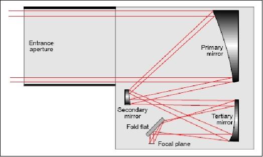
SPIRIT-III (Spatial Infrared Imaging Telescope)
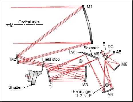
SPIRIT-III was developed and built at SDL (Space Dynamics Laboratory) of Utah State University. The instrument package is the primary sensor system on MSX with the objective to perform midcourse surveillance functions, collect target and background phenomenology data, and to demonstrate advanced cryogenic sensor technologies. The requirements are to characterize Earth-limb and celestial backgrounds and measure the spectral, spatial, temporal, and intensity parameters of stars and upper atmospheric phenomena, including airglow and aurora. The goal is also to characterize the signatures of selected targets operating against natural backgrounds and to assist investigators in identification and evaluation of the chemical and physical properties of the upper atmosphere on a global scale.
The instrument consists of an off-axis re-imaging telescope with a 35 cm diameter unobscured aperture, a six-channel high-spectral-resolution Michelson interferometer, a five-band scanning radiometer, and a cryogenic dewar/heat exchanger (the dewar cools the telescope, radiometer and spectrometer, the cryogen is expected to last for 15 months, cryogen volume of 944 liter). Total instrument mass = 967 kg; size = 107 cm diameter x 360 cm in length. 25)
Note: SPIRIT-I and -II were instruments (FTIR spectrometers only) flown on sounding rockets in the late eighties and in 1991 - as part of the SDIO (Strategic Defense Initiative Organization) heritage.
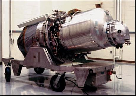
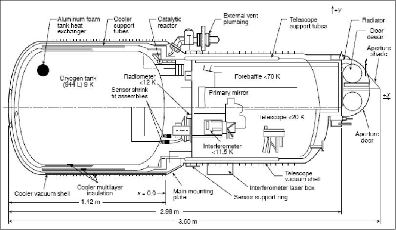
The sensor components are conductively cooled and maintained at operating temperatures via thermal links, connecting them to the solid-hydrogen tank of the cryostat subsystem. Power consumption ranges from 50 to 410 W, depending on the mode of operation. The optical components of SPIRIT-III telescope operate at temperatures ranging from 10 to 20 K. The cryosat subsystem was built by Lockheed Martin of Palo Alto, CA under contract to SDL.
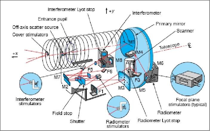
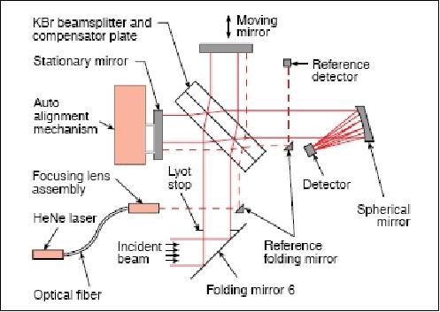
Optics (Figure 13): The telescope has three sections: the afocal foreoptics (M1, M2, M3), the radiometer re-imaging optics, and the spectrometer collimating optics. The foreoptics use an off-axis all-reflective design. An auto-collimator measures telescope alignment with respect to the S/C attitude system optical bench to an accuracy of 5 µrad. The Michelson interferometer (Fourier-transform spectrometer) has six Si:As detectors operating at 10.5 to 11.0 K. It collects double-sided interferograms in six spectral bands with programmable resolution of 2, 3.9, or 20 cm-1 over sample times of 4.2 s, 2.2 s, and 0.55 s.
Radiometer
The radiometer has five Si:As focal plane detector arrays of 8 x 192 pixels each, operating between 11 and 12 K. It collects data in six passbands with a spatial resolution of 90 µrad. The scan mirror can remain fixed or can operate at a constant scan rate of 0.46º/s with programmable scan fields of regard of 1º x 0.75º, 1º x 1.5º, or 1º x 3º. The radiometer focal plane assembly employs a combination of dichroic and bandpass filters to allow simultaneous measurements in bands A, D and E and or in bands B and C. Table 3 lists the four operational modes and provides actual values for the radiometer field of regard (FOR). - Earthlimb observations of SPIRIT-III include an experiment to measure chlorofluorocarbons and nitric acid. Channel 5 (10.6-13 µm) of the FT spectrometer collects data in the altitude range from 10 to 40 km. Dominant emissions in this channel include nitric acid, CFC compounds, ozone, and the thermal signature of stratospheric aerosols.
The SPIRIT-III interferometer-spectrometer focal plane consists of six detector elements (Figure ) physically separated on individual substrates with no overlapping fields of view. The detectors are similar to the radiometer detectors in composition but are significantly larger. They are arsenic-doped silicon, blocked impurity-band conductor detectors with spectral responsivity ranging from 2.5 to 28.0 µm. The focal plane arrays were provided by Rockwell International under contract to SDL.
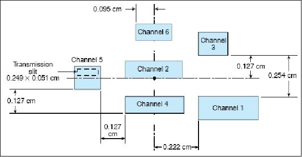
FT Spectrometer Passbands | Radiometer Passbands | ||||
Channel | Passband (µm) | Band | Passband FWHM (µm) | Active Columns | Noise equivalent radiance for |
1 | 17.2 - 28.0 | A | 6.03 - 10.91 | 8 | 1.1 |
Parameter/Function | Mirror-hold | Mirror-scan 1 | Mirror-scan 2 | Mirror-scan 3 (3.0º) |
Scan rate | 0.05868º/s | 0.46º/s | 0.46º/s | 0.46º/s |
Scan period (one full, double scan cycle) | N/A | 3.66 s | 7.32 s | 14.65 s |
5-color scan FOR | drift position limited | 0.426º x 0.99º | 1.268º x 0.99º | 2.953º x 0.99º |
Color-set scan FOR | drift position limited | 0.842º x 0.99º | 1.685º x 0.99º | 3.369º x 0.99º |
Sampling rate | 72/360 | 72/360 | 72/360 | 72/360 |
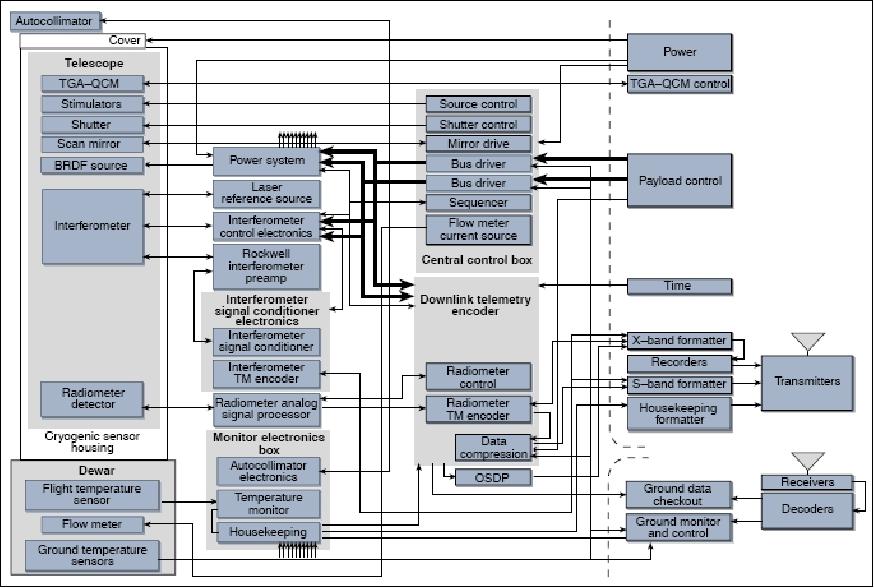
Legend to Figure 17: Heavy lines indicate paths for spacecraft control data bus. (TGA = thermogravimetric analysis, QCM = quartz crystal microbalance, BRDF = bidirectional reflectance distribution function, and OSDP = Onboard Signal and Data Processor).
UVISI (Ultraviolet/Visible Imaging and Spectrographic Imaging)
UVISI is a hyperspectral suite of nine instruments, designed by APL. The primary objective of UVISI is to collect data on celestial and atmospheric backgrounds; secondary objectives include target characterization and contamination observations in conjunction with the contamination instruments.
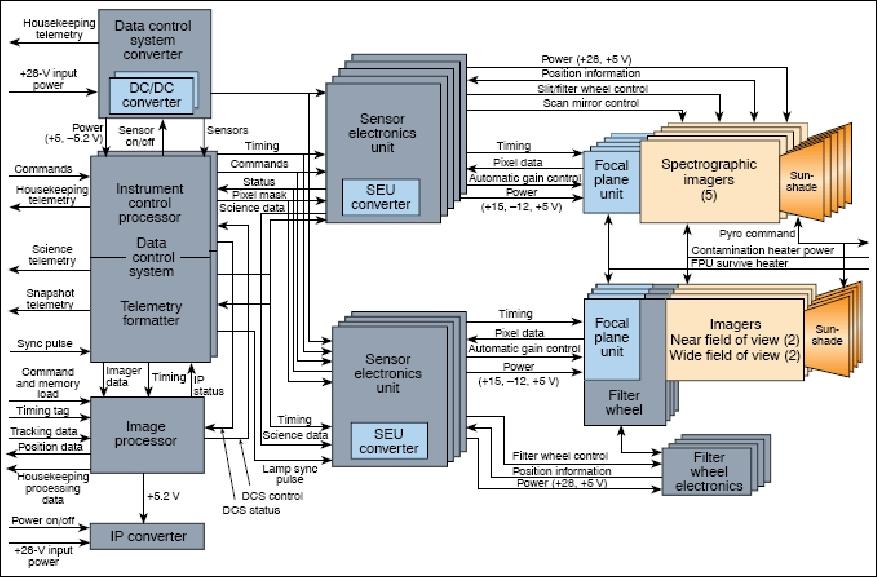
The UVISI sensor system consists of five SPIM (Spectrographic Imager) instruments, four imagers, and a set of instrument electronics that provide control functions and image processing capabilities (Figure 19). The imagers include two WFOV (Wide-Field-of-View) and two NFOV (Narrow-Field-of-View) sensors in the UV and VIS spectrum, respectively. Together the 5 SPIMs as well as the 4 imagers cover an overlapping spectral range from 110 nm (UV) to 900 nm (VNIR). See Figure 20 and Tables 4 and 5. 26)
The nine instruments share a common boresight with each other, with the SPIRIT-III IR radiometer, and with the SBV instrument.
Each UVISI sensor has its own radiation-hardened 80C85-based local controller or SEU (Sensor Electronics Unit). The functions of the SEU include CCD and analog-to-digital timing control; image intensifier gain control; filter wheel, scan mirror, and slit wheel mechanism control; command and telemetry communications with the DCS (Data Control System); data collection from the FPU (Focal Plane Unit); and secondary power generation and distribution to the FPUs and mechanism controllers.
The DCS is the single interface for the operation of all nine UVISI sensors via the spacecraft command and data handling systems, and the UVISI imagers interface via the image processor. It is one of two redundant packages in the instrument. The DCS commands the sensor's operational mode and its on and off sequence. It is designed to process the sensor data to match the bandwidth of the sensors to the available spacecraft telemetry bandwidth on the 16 kbit/s, 1Mbit/s, and prime science 5 or 25 Mbit/s telemetry links. This subsystem synchronizes all sensor data collection in either the 2 or 4 Hz frame rates.
The UVISI instrument contains an image processor that selects and processes images from one of the four imaging sensors. Its purpose is to provide the spacecraft tracking processor with information needed to complete closed-loop tracking of targets of interest. From an analysis of the contents of each image, the image processor generates a list of potential targets. This list is sent to the MSX tracking processor, where its data are input to a tracking loop.
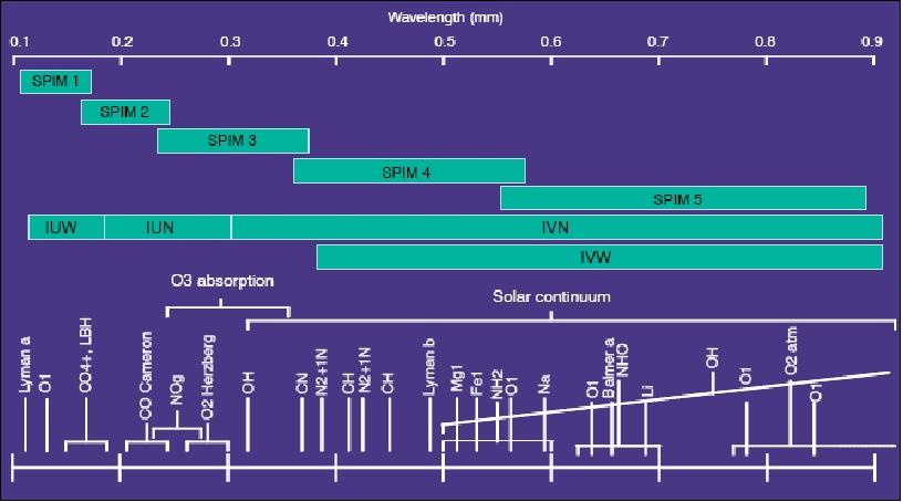
UVISI SPIMs: All five SPIMs feature an all-reflective off-axis parabolic design (external sunshade, scanning mirror, slit/filter, collimating mirror, dispersive grating, and an intensified CCD focal plane) in which selectable slits provide spectral resolutions between 0.5 nm to 4.3 nm. The SPIM image planes have programmable spectral dimensions with 68, 136, or 272 pixels and programmable spatial dimensions with 5, 10, 20, or 40 pixels. A scan mirror sweeps the slit through a second spatial dimension and generates a spectrographic image once every 5, 10, or 20 seconds.
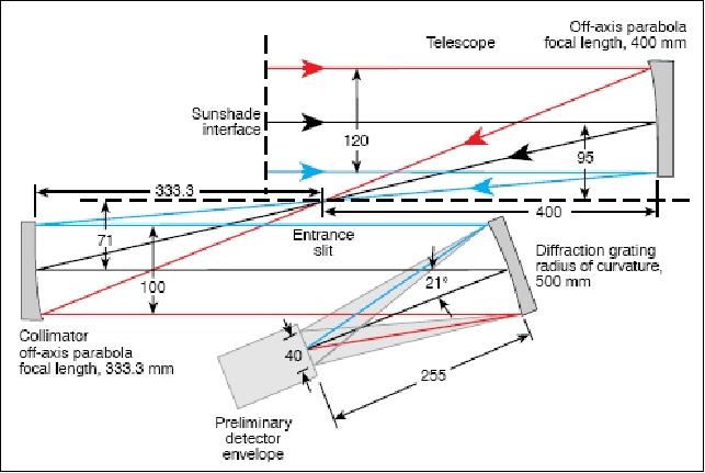
The SPIM CCD detector plane collects an image of the slit length in one direction and spectral information in the other (Figure 23). One spatial dimension is resolved along the slit and the other spatial dimension information is obtained by moving the FOV either 0.05º or 0.1º before recording another observation. It takes about 10 s to complete a 1º x 1º image in either 10 or 20 steps. The five-position slit/filter mechanism provides two slit sizes (1.0º x 0.10º and 1.0º x 0.05º) and various blocking filters that eliminate extraneous spectral orders and long-wavelength contaminants.
Note: The spatial resolution of the SPIMs is driven by the point-spread function in one direction (along the slit) and by the point-spread function and the mirror step size in the other direction. For the 0.05º mirror steps one can assume that it is driven by the point-spread function in both directions, and is about 0.85 mrad. The spatial resolution is diminished by using the 0.1º steps or by reducing the number of bins in the readout, by co-adding 2, 4, or 8 adjacent pixels. This is to reduce the bandwidth requirement by trading spatial resolution, spectral resolution and frame rate. The nadir resolution is 0.85 mrad x 900 km ≃770 m. Nadir FOV is 17 mrad (1º) x 900 km ≃15 km x 15 km.
Instrument | Passband Range (nm) | Resolution Δλ (0.10º slit) | Resolution Δλ (0.05º slit) | No. of Bins |
SPIM1 | 113-173 | 0.8 nm | 0.5 nm | 68, 136, or 272 |
The SPIM electronics (Figure 19) perform pixel-summing operations (programmable) on the 40 x 272 element SPIM focal plane array, yielding 40, 20, 10, or 5 bins in the spatial direction, and 272, 136, or 68 bins in the wavelength direction. The pixel resolution is 14 bit.
Note: The bins are formed in the SPIM electronics by co-adding 1, 2, or 4 adjacent pixels; this is done to reduce the data bandwidth requirement in cases where UVISI is not the principal instrument, or higher frame rates are needed which can be traded off against resolution. For the case of 136 and 272 bins, the bins overlap; for the case of 68 bins, the bins are noncontiguous.
With a dynamic range of 1011, UVISI has the capability to obtain data ranging from noontime surface-reflected visible radiation to observations of a diffuse UV celestial background. Objective and applications: generation of spatial/spectral maps of various objects and scenes; prime SPIM observations include the atmospheric dayglow and nightglow, aurora, stars, zodiacal light, and plume contrails. When suitably inverted, SPIM radiance measurements can reveal atmospheric properties such as species concentrations, temperatures, and altitude profiles. SPIM investigations of auroral radiances can provide estimates of fluxes and energies of precipitating particles that cause auroral emissions.
UVISI Imagers
The four imager suite consists of: external sunshade, imaging optics, filter wheel and drive motor, and intensified CCD focal planes. Three of the four imagers employ all-reflective optics. Both NFOV imagers use a Cassegrain design; the UV WFOV imager uses an off-axis three-mirror design.
The commandable filter wheel in each imager houses three bandpass filters on a neutral-density (ND) filter. In case of the visible WFOV imager, a lens is substituted for one of the filters. This lens is used to focus the near-field backscattered emissions from the xenon flashlamp as part of the MSX contamination experiment. The filter bands were chosen for specific objectives. For example, the UV-NFOV 200-230 nm filter is used to observe the NOy bands in airglow measurements. The UV-WFOV 117-127 nm filter is used for viewing Lyman-α emission from hydrogen in the geo-corona, from auroral hydrogen precipitation, or from outgassing of the SPIRIT-III cryogen. Each imager has a focal plane CCD array of 256 x 244 pixels with 12 bit resolution. The imager nadir resolutions are:
• NFOV: 0.09 mrad x 900 km ≃80 m
• WFOV: 0.82 mrad x 900 km ≃750 m
The limb resolutions can be calculated from geometry, given a tangent height.
Instrument | UV-NFOV | UV-WFOV | VIS-NFOV | VIS-WFOV |
FOV | 1.28º x 1.59º | 10.5º x 13.1º | 1.28º x 1.59º | 10.5º x 13.1º |
Resolution (IFOV) | 90 µrad | 820 µrad | 90 µrad | 820 µrad |
Passband (nm) | 180-300 | 110-180 | 300-900 | 380-900 |
ND filter | 10-3 | 10-3 | 10-4 | 10-4 |
The UVISI image processing system can acquire and isolate likely targets in an image FOV and communicate their positions to the MSX flight processor, which in turn points the satellite in a "closed-loop" fashion. The term "target" may refer to either a point source such as a star, to another satellite, or to an extended source such as an auroral or cloud-top feature. The processor software performs initialization and tracking functions that include filtering, smoothing, thresholding, and centroiding. The image processor seeks targets based on an a priori target description file containing weights for numerous target features such as size, brightness, and location. The image processor then transforms target locations from UVISI pixel coordinates to S/C coordinates and passes them on the MSX flight processor, which performs Kalman filtering of other targeting inputs to select "true" targets for observation.
The MSX/UVISI Stellar Occultation Experiments 27)
A primary means of monitoring the atmosphere on a global scale is remote sensing of Earth from space, and occultation methods based on observing changes in a star's spectrum as it sets through the atmosphere have proven valuable in this endeavor. Two occultation techniques — focused respectively on atmospheric extinction and refraction — have been treated separately historically, but the combination of the two offers the possibility of higher accuracy, greater altitude coverage, and simultaneous measurement of primary and trace gases, both of which are important in the chemical balance of the atmosphere. Using data from the UVISI (Ultraviolet and Visible Imagers and Spectrographic Imagers) on the MSX (Midcourse Space Experiment) satellite, the team has developed a combined extinctive/refractive stellar occultation technique that relates the changes in measured stellar intensity to the height-dependent density profiles of atmospheric constituents and have demonstrated its viability for retrieving both primary and trace gases through the analysis of approximately 200 stellar occultations. This self-calibrating technique is broadly applicable and suitable for measurement of gases that are otherwise difficult to quantify on a global basis.
Stellar occultation is one of the most promising techniques to meet the needs of atmospheric scientists, policy makers, and enforcement agencies tasked with understanding and regulating man-made contributions to the trace gas atmospheric budget. Occultation techniques have been used for many years to study the atmospheres of Earth, other planets, and their satellites. Because these techniques are generally based on relative measurements (i.e., compared to measurements in the absence of the occulting atmosphere), they tend to be less sensitive to instrument degradation and changes in calibration than other remote sensing methods. Although these techniques are easy to implement in principle, technical hurdles exist. As these challenges have been overcome, occultation techniques have proven to be an excellent means of exploring the overall structure of both terrestrial and planetary atmospheres.
Using occultation methods to probe Earth's lower atmosphere is complicated by the effects of both refraction and extinction as light passes through the densest part of the atmosphere. To demonstrate a new approach to this challenge, the project team took advantage of the UVISI suite of instruments onboard the MSX spacecraft to conduct stellar occultation experiments in which techniques were combined, suited to measuring refraction and extinction independently into a single, self-consistent occultation method that leverages the benefits of both techniques. This demonstration led to the development of an instrument concept suitable for flight on a small space platform.
The potential measurement capabilities of this combined stellar occultation technique are illustrated in Figure 26. The left panel shows the retrievable altitude ranges for several gas and aerosol constituents in the terrestrial atmosphere that can be measured over far-UV to visible wavelengths, whereas the right panel shows the altitude ranges for gases that can be measured in the near-IR. These altitude ranges are derived from an analysis of the extinction spectra for the various species (a term commonly applied to atmospheric constituents) and the capabilities of an instrument optimized for their measurement, particularly in the lower atmosphere where refraction effects must be accounted for in extinctive occultation observations.
Legend to Figure 26: The left panel shows the retrievable altitude ranges for several species in the terrestrial atmosphere that can be measured over the wavelength range of 100–900 nm. The blue bars represent ranges that are generally measurable under all conditions, whereas the red bars represent ranges that vary depending on the atmospheric conditions (e.g., night/day, presence of high-altitude clouds) and the target star involved (e.g., spectral type, magnitude). Colored bars along the right y axis denote the altitude ranges of various atmospheric regions. The right panel shows the retrievable altitude ranges for several terrestrial species that can be measured if coverage is extended into near-IR wavelengths: 0.8–2.5 µm (blue bars) or 0.8–5.0 µm (blue+red bars). In both panels, the actual lower limits of the altitude ranges are determined by cloud-top heights at the time of the occultation; the limits shown are for clear skies. Note that the upper limits on CO2 and O3 in the right panel are truncated to 50 km to allow the panel to focus on the lower altitudes.
The Stellar Occultation Technique
Two general categories of occultations exist: extinctive and refractive. In both, radiation from a source is affected by physical processes in the atmosphere, and measurements of the outgoing radiation are used to infer atmospheric properties.
1) Extinctive stellar occultations:
The principles of extinctive stellar occultations are similar to those of classical absorption spectroscopy. As shown in the upper left of Figure 27, a star is used as the light source, a spectrometer serves as the detector, and the intervening atmosphere acts as the absorption cell. The spectrometer is most commonly mounted on a spacecraft but may also be on Earth's surface or on a balloon, in which case the effective absorption path is half that shown in the figure. Starlight passing through the atmosphere is attenuated because atmospheric constituents either absorb or scatter the incoming light.
Although the physical process involved is different, the net effect of extinction by scattering (molecular/Rayleigh or aerosol/Mie scattering) is similar to that by absorption (i.e., scattering "out of the beam" reduces light intensity far more than scattering "into the beam" increases it); therefore, the term extinction as used here refers to any absorption or scattering process. As the line of sight to the star moves deeper into the atmosphere, the light is progressively attenuated because the effective extinction path length increases. At the same time, changes in the densities of the species responsible for extinction along the path are recorded in the measured spectra. The ratio of an attenuated spectrum, I, to the unattenuated spectrum, Io, is referred to as the atmospheric (or stellar) transmission and is the fraction of light that passes through the atmosphere as a function of wavelength. The minimum altitude to which a ray penetrates is referred to as the tangent point height or tangent point altitude of the measurement, or more simply as the tangent point. Note that in this article, we use altitude to refer to the actual altitudes relevant to atmospheric density profiles, whereas tangent point altitude or height is used to refer to the minimum altitude of an observation. The distinction is subtle but will be made clear as we discuss the observations.
Because the extinction cross sections of most species are wavelength dependent, spectral measurements of the transmission represent a "fingerprint" of the relevant species. Thus, they are diagnostic of the atmospheric composition, and densities of the species involved can be determined from the observed transmission spectra. Figure 28 illustrates the wavelength dependence of the altitude at which the density of several species results in a specific level of extinction, in this case the τ = 0.1 level. Extinction in the atmosphere is generally proportional to the function exp(–τ(λ)), where λ is the wavelength and τ is referred to as the optical depth; thus, τ = 1 refers to the point in the atmosphere at which the total flux from a star at a given wavelength has decreased to 1/e of its unattenuated value. Because the transmission is related to the optical depth, this figure is also illustrative of the range of altitudes over which the density profiles of such species may be inferred from transmission spectra. Extinction as a function of wavelength and altitude for the species in Figure 28 and for other species form the basis of the altitude ranges illustrated in Figure 26. With a properly designed instrument, accurate retrievals can generally be carried out over transmissions ranging from 1 to 99% (τ ranges of roughly 0.01–4.5).
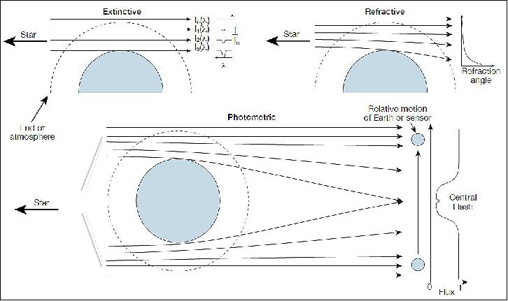
Legend to Figure 27: The upper left panel shows the geometry of an extinctive occultation, in which the flux Io(λ) from a star is progressively attenuated as the line of sight to the star moves deeper into the atmosphere. The ratio of the measured flux I at each point to the stellar flux is I/Io, known as the atmospheric (or stellar) transmission. Transmission values run from 0 (full extinction) to 1 (no extinction) and are a function of wavelength because the extinction by the atmosphere depends on the wavelength. The upper right panel shows the geometry of a refractive occultation, in which the angle between the observed ray and the unrefracted ray (the incoming stellar ray) is measured. The deeper in the atmosphere the line of sight penetrates, the larger the measured refraction angle will be. The lower panel shows the geometry of a photometric occultation, which is a variant on the refractive occultation. In this case, rather than measure the refraction angle of the star, the total flux from the star is measured. As the rays from the star diverge due to refraction, the relative flux measured at the sensor drops from a value of 1 outside the atmosphere to 0 when the star is blocked by the planet. This is because diverging rays fall outside the sensor field of view, and the greater the divergence, the less flux that is measured. The central flash often seen in the total flux is caused by the convergence of rays refracted around opposite sides of the planet even though the star itself is completely blocked.
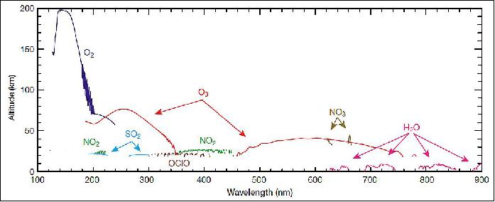
Legend to Figure 28: Because extinction is generally proportional to the function exp(–τ), the τ = 1 level is that point in the atmosphere at which the total flux from a star at a given wavelength has decreased to 1/e of its unattenuated value. Because the extinction character of different atmospheric species varies with wavelength, plots such as this are helpful in designing occultation instruments because they highlight where extinction is most likely and indicate the altitude ranges in the atmosphere that it is possible to probe (e.g., Figure 26).
The possibility of using stars as the source in an extinctive occultation observed by a space-based platform was first suggested by Hays and Roble. 28) The first stellar occultation measurements of the terrestrial atmosphere came a few years later when a spectrometer on the OAO-2 (Orbiting Astronomical Observatory) satellite was used to infer density profiles for molecular oxygen (O2) and ozone (O3) in the thermosphere and upper mesosphere. Since OAO-2, extinctive stellar occultations have yielded densities for a number of species in Earth's atmosphere, including O2, O3, NO, NO2, NO3, N2O, H2, CH4, CO, H2O, Cl, and OClO.
2) Refractive stellar occultations:
Refractive stellar occultations occur because density gradients in the atmosphere lead to refraction, or bending, of the path of incoming starlight. This results in the light following curved paths through the atmosphere, which leads to differences between the star's true (geometric) and apparent (refracted) positions. Measurements of the degree to which the path of the incoming starlight is changed provide the bulk properties of the atmosphere (i.e., total density, pressure, temperature). Pannekoek first realized the potential of refraction for studying planetary atmospheres, but roughly 50 years would pass before technology progressed to the point that useful observations could be made.
The primary refractive stellar occultation technique is the photometric approach (see the lower panel in Figure 27), which involves visible-light observations of the occultation of stars by a planetary atmosphere using ground, aircraft, or space-based telescopes. This approach has been applied primarily to the study of the atmospheres of the other planets. As a star passes behind a planet, light rays passing through deeper regions of the atmosphere are refracted more than rays at higher altitudes. This results in a divergence of the incoming parallel light from the star. At the detector, the divergence appears as an attenuation of the light as a function of time (referred to as refractive attenuation) as more and more of the total flux from the star is refracted out of the field of view of the sensor. Photometric observations of this attenuation yield the so-called occultation light curve, which may be inverted to retrieve the atmospheric density, pressure, and temperature.
Often, these photometric occultations yield light curves that exhibit rapid fluctuations in intensity. These fluctuations are caused by a refractive phenomenon known as scintillation, which arises from small-scale variations in the density profile at points along the line of sight. Such variations may be caused by atmospheric turbulence or by the presence of atmospheric waves. When combined with models of such variations, measurements of the scintillation have proven useful in inferring the small-scale atmospheric structure.
Earth's lower atmosphere: Historically, extinctive stellar occultations have been applied to high altitudes for three reasons. First, the species involved (e.g., O2 and O3 for Earth) have strong spectral signatures at UV wavelengths, which are completely absorbed by the atmosphere before the lower altitudes are reached. Second, the presence of atmospheric emissions (e.g., airglow) from other species that occur in the instrumental bandpass used in the occultation experiment leads to an additional source that competes with the stellar signal. Once the line of sight to the star has passed below the atmospheric level of such emission, which ranges in altitude depending on the wavelength and species involved, the emission is always present as a contaminating source. Separation of the stellar and emission sources is therefore necessary and can be complicated. Finally, there are no significant refractive effects at high altitudes, allowing a straightforward interpretation of the observed transmission.
Refractive stellar occultations have been limited almost exclusively to the study of other planets. The primary reason for this is that the long distances involved allow for a greater separation of the diverging rays and a more easily measured change in the stellar intensity. At the same time, the choice of visible wavelengths for these occultations generally excludes the need to consider extinction of the starlight within the atmosphere itself.
These extinctive and refractive methods, however, are complementary, and consideration of both processes would allow stellar occultation measurements to probe a larger altitude range more accurately than either one taken individually. In particular, the idea of using extinctive stellar occultations to probe Earth's lower atmosphere by considering the effects of refraction on the measurements was first proposed by Hays and Roble (Ref. 28). They favored stellar occultations over solar occultations, which have been the primary occultation method of studying Earth's lower atmosphere, for a number of reasons. Stellar occultations are not limited to the terminator and allow for hundreds of occultations per day with near-global coverage versus the 30 or so daily using solar occultations. Stellar occultations can also yield higher vertical resolution owing to the point nature of the source; the Sun subtends an angular range of half a degree, which corresponds to about 30 km in altitude.
Solar occultations do yield higher signal-to-noise ratio observations owing to the intensity of the Sun relative to stars, and solar occultations are generally immune to the effects of atmospheric emissions because the Sun is so much brighter than the atmosphere. However, in the lower atmosphere where refraction is significant, stellar occultations have the advantage over solar occultations in that the refractive effects can be treated more easily for stars (as point sources) than for the Sun (as an extended source).
MSX/UVISI Stellar Occdultations
The research team took advantage of the capabilities of MSX and UVISI to test the suggestions of Hays and Roble (Ref. 28) and thereby demonstrate the viability of using stellar occultations for the retrieval of atmospheric composition, particularly in the lower atmosphere. Although the MSX spacecraft and the UVISI suite of instruments were not specifically designed for stellar occultations, their combination fortuitously satisfied the stringent requirements necessary to conduct these experiments. Rather than simply use models or climatological information to treat the effects of refraction on the extinctive measurements, the MSX/UVISI experiments focused on a combined extinctive and refractive stellar occultation technique in which SPIMs (Spectrographic Imagers) were used to measure the wavelength-dependent atmospheric extinction of starlight while a co-aligned imager [IVN (Imager/VIS/NFOV)] was used to measure the atmospheric refraction along the same line of sight.
The key element in this new approach to stellar occultations was the direct measurement of the refraction angle of the star at visible wavelengths, as suggested by Jones et al. Although simple in concept, this method of refraction angle measurement has previously been used in only a few, mostly serendipitous, instances.
The MSX/UVISI experiments represent the first systematic implementation of the technique. The refraction angles themselves are used to infer atmospheric refractivity and subsequently the bulk atmospheric density, pressure, and temperature. Although the temperature profiles determined from such measurements are unlikely to ever be as accurate as profiles derived from radio occultation methods such as those used in GPS/MET (Global Positioning System/Meteorology), the advantage of this visible-light technique is that the refraction angles are measured simultaneously along the same line of sight as the extinction measurements.
By simultaneously measuring both refraction and extinction effects on the stellar spectrum, the extinction measurements were able to probe the atmospheric composition accurately at the low altitudes where refraction is significant. Measurements of refraction provided the actual light path through the atmosphere and the bulk atmospheric properties, both of which are necessary to determine extinction accurately in the refractive region of the lower atmosphere. More importantly, knowledge of the total density profile allowed the effects of Rayleigh scattering in the transmission spectra to be handled accurately. The simultaneous measurement of both constituent and total density profiles also allowed for direct calculation of volume mixing ratios, a key quantity that typically has to be inferred and is therefore subject to increased uncertainty.
The design of the MSX/UVISI stellar occultation experiments and the associated extinction and refraction retrieval algorithms are discussed in detail in a three-paper series. 29) 30) 31) A full discussion of the combined technique, the development of the retrieval algorithms, and a rigorous assessment of the uncertainties may be found in these papers. In this article, we present an overview of the technique and analysis methods along with a summary of several results that highlight the potential of the combined extinctive and refractive stellar occultation technique for studying Earth's atmosphere.
Typical MSX/UVISI Occultation Event
The geometry of a typical MSX/UVISI stellar occultation event is shown in Figure 29. The star was acquired at high tangent altitudes and the boresights of the UVISI instruments remained fixed on the star's inertial position during the entire occultation. The entrance slits to the five spectrographs were held vertical with respect to the horizon. Several hundred unattenuated Io spectra were obtained at high altitudes before any atmospheric effects began. As the star set through the atmosphere, its spatial position in the spectrograph images was unchanged until refraction set in at altitudes below roughly 35 km, after which the image drifted vertically up the slit until it slowly disappeared from the field of view. For a star inertially fixed in the center of the slit, roughly 0.5º of motion due to refraction could be observed before the star's image reached the edge of the frames, corresponding to apparent tangent point altitudes of 7–8 km.
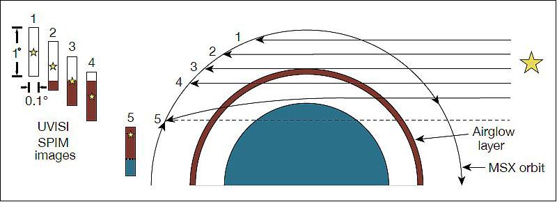
Legend to Figure 29: The UVISI instrument is oriented so that the slit is vertical with respect to the atmosphere horizontal. The center of the slit is fixed on the star's inertial position throughout the occultation; therefore, the star itself can refract up to 0.5° before disappearing from the field of view. The 1° field of view in the vertical direction corresponds to ~60 km at the limb. The superposition of the background airglow
(magenta) and stellar signals once the line of sight has passed through the airglow layer is illustrated. The minimum height of the solid rays above Earth's surface (blue) reflects the apparent tangent point altitude, whereas the dashed line between the spacecraft and the star is an example of the geometric tangent point altitude, which can be negative. In the absence of refraction, the two quantities are equal.
As seen in path 5 of Figure 29, the direct line of sight to the star (dashed line) at that point actually had a tangent point altitude below the horizon. The tangent point altitude of the direct line is referred to as the geometric tangent point altitude and can be negative. When refraction is not important (i.e., above 35 km), the apparent and geometric tangent point altitudes are the same.
As illustrated in Figure 29, airglow emissions are an issue. These first appear in the bottom edge of a spectrographic slit as it descends through the altitudes at which the emissions originate (e.g., the airglow layer). The peak in the emission layer signal will continue to move up the slit, eventually disappearing above the top edge. However, once the line of sight passes through the airglow layer, the stellar signal is superimposed on an ever-present background airglow signal. Because each spatial pixel covers a field of view of ~0.025° (about 1.5 km projected onto the limb), the UVISI SPIMs are essentially used as large-aperture photometers (~100 cm2) with an effective field of view of 0.1° x 0.025°. With a maximum star setting rate of roughly 0.07°/s (~3 km/s), the limb airglow emission at a given tangent point altitude is sampled for approximately 10 s. On the ground, this multiple sampling of the airglow allows us to "shift" the SPIM pixels spatially and co-add them in a manner similar to that used for a time-delay and integration system, thereby improving the signal-to-noise ratio of the observations and subsequent accuracy of the separation of the stellar and airglow signals.
Figure 30 shows a series of images acquired at different times during a typical MSX/UVISI occultation to illustrate the extinction of stellar light with altitude. The panels show composite SPIM spectral images together with an IVN image acquired simultaneously. Scene brightness is represented by a color scale as a function of geometric tangent altitude (y axis) and wavelength (x axis) in the SPIM images. The star appears as a bright, narrow, horizontal band in the composite SPIM images because it is a point source emitting a continuous spectrum at all wavelengths, whereas the airglow signal covers an extended portion of the slit vertically owing to the diffuse nature of the airglow emission. The ragged horizontal edges of the SPIM images result from small, well-known misalignments of the five SPIM boresights plus corrections for optical aberrations when referencing the stellar signal at each wavelength to a common tangent point altitude. Black areas in Figure 30 correspond to altitudes outside the SPIM fields of view, and a decrease in the SPIM 5 sensitivity results in the weak signal at the longest wavelengths of the spectral range. The star of interest is the bright dot near the center of each IVN image.
The data in Figure 30a correspond to a geometric tangent altitude of 245 km. There is essentially no atmospheric attenuation of the star at this altitude; however, several airglow emissions are visible in the spectrum [e.g., geocoronal H Lyman α at 121.6 nm, nightglow O(1S) "green line" at 557.7 nm, and nightglow O(1D) "red lines" at 630.0 and 636.4 nm]. Spectra from such altitudes and higher provide the unattenuated stellar Io spectra needed to determine the atmospheric transmission.
In Figure 30b, the line of sight has descended to a tangent altitude near 95 km. Complete attenuation of the star by O2 is evident in the Schumann-Runge continuum and bands shortward of 200 nm, whereas absorption by O3 in the Hartley/Huggins bands is just beginning near 255 nm. Emissions in Earth's mesospheric airglow layer are now visible [e.g., O(1S) "green line," O2 Atmospheric (0-0) band at 762 nm, several OH Meinel bands in the near-IR]. The mesospheric emissions cover only the lower portion of the SPIM images because the upper part of the slit still views tangent heights above the mesospheric airglow emission layer. Even though the stellar signal short of 200 nm is gone, the H Lyman α geocoronal line is still present owing to emission that originates above the tangent point and extends into the geocorona. From the geometry of Figure 29, it can be seen that this "near-field" source also exists for the airglow layer, explaining why many of the airglow emissions are only moderately attenuated as the occultation progresses.
Figure 30c shows the image when the star has reached a geometric tangent height of 20 km. In the lower stratosphere, the O3 column density has increased to the point that absorption in the Hartley/Huggins bands is complete, whereas absorption in the relatively weak Chappuis band near 600 nm has now become significant. The star has also moved in the SPIM and IVN images, shifting slightly upward as a result of refraction. Note that the second star in the upper right corner of the IVN image is at a higher tangent height and has not yet been refracted. Finally, Rayleigh extinction, refractive attenuation, and scintillation effects are becoming increasingly important as evident in the overall reduction of the stellar signal.
In Figure 30d the geometric tangent altitude of the star has descended to 0 km, but refraction is sufficient to keep the star visible above the horizon. The refractive shift of the star's position is evident not only in the IVN image but also in the SPIM data where the bright line delineating the stellar spectrum has moved upward relative to the slit center, which is fixed on the star's inertial position. The star's apparent tangent height is roughly 13 km as shown in SPIM 5. The stellar signal continues to weaken and is visible only at the longer wavelengths. Both Rayleigh scattering and refractive attenuation act to block the majority of the stellar signal at tropospheric altitudes. At the same time, the relative constancy of the "near-field" airglow emissions from panel to panel results in a comparable, or even brighter in the case of 762 nm, signal relative to the star. This ultimately results in a decreased signal-to-noise ratio in the wavelength channels of the stellar transmission spectra contaminated by airglow once the two signals are separated.
Each MSX/UVISI occultation consists of images such as those presented in Figure 30. Before the atmospheric retrievals, the spectral images must be processed to remove a number of instrumental effects (e.g., changes in gain with altitude, dark subtraction), and the stellar spectra must be separated from the contaminating airglow background. Accomplishing this requires knowledge of the true stellar position in the SPIM images, which is calculated from the measured position of the star in the IVN images and known relationships in the relative alignments of the various instruments (thereby emphasizing the need to both know and maintain the relative co-alignment of the SPIMs and imager).
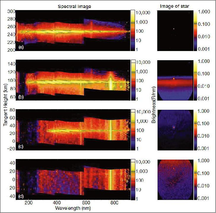
Legend to Figure 30: The images on the left are from the spectrographic imagers and illustrate how the star's spectrum (the bright horizontal line in the center of each image) is attenuated as a function of wavelength (left to right) and altitude (top to bottom). Note that the tangent height scale changes with each panel to be centered on the tangent height of the unrefracted star (i.e., its inertial position). Thus, the spectrum has moved "up" relative to the panel center in the final panel. Bright lines in the vertical direction are emissions from Earth's atmosphere (i.e., the background airglow). The images on the right are from the IVN imager and show the position of the star corresponding to the spectrographic imager measurements on the left. Note that the star moves up away from the image center as refraction begins. The refraction angle is the angle between the center and measured positions (Ref. 27).
SBV (Space Based Visible) Sensor
The SBV optical camera was designed and built by the MIT Lincoln Laboratory (MIT/LL) under the ACTD (Advanced Concept Technology Demonstration) program. The objective is to collect data on celestial target signatures (stars) in the VIS range and to perform above-the horizon surveillance demonstrations (cataloging of resident space objects). It uses a broadband visible wavelength detector and signal processor to automatically detect space objects, such as intercontinental ballistic missile targets and satellites, from their reflected sunlight. The goal of the SBV instrument is to provide high-performance search, detection, tracking, and data gathering on space objects to support both midcourse surveillance and space surveillance missions.
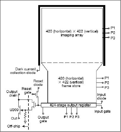
The instrument incorporates a 15 cm aperture off-axis, re-imaging, all-reflective telescope, a thermo-electrically cooled (front-illuminated) bare CCD focal plane, and electronic subsystems. The focal plane consists of four CCDs with 420 x 420 (27 µm) pixels each, Use of MIT/LL CCID7 frame-transfer visible-light CCDs, which were specifically developed for space surveillance - where CCID7 (Charge-Coupled Imaging Device 7). A primary reason for selecting the CCID7 imager is its unique combination of high charge transfer efficiency and low readout noise. 32) 33)
Spectral range | 0.3 - 0.9 µm |
Spatial resolution (IFOV) | 60 µrad |
FOV | 1.4º x 6.6º |
Aperture, focal ratio | 15 cm, f/3 |
Focal Plane Array (FPA, four CCDs) | 420 x 1680 pixels |
Frame times | 0.4 s, 0.5 s, 0.625 s, 1.0 s, 1.6 s, 3.125 s |
Instrument mass, power | 78 kg, 68 W |
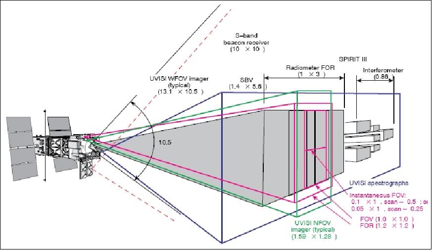
Legend: The SPIRIT-III interferometer FOV is completely outside of the field of regard (FOR) of the SPIRIT-III radiometer. The two are placed in context by the UVISI wide field of view (WFOV) imagers, IUW and IVW. The UVISI spectrographic imagers (SPIMs) and the SPIRIT-III radiometer have instantaneous FOVs that are perpendicular to each other. Both the UVISI SPIMs and the SPIRIT-III radiometer use a scan mirror to achieve the desired FOR (Ref. 5).
Contamination Experiments
MSX carries in addition a suite of contamination instruments with the objective to characterize the molecular and particulate environment onboard and around the spacecraft (all APL sensors). This suite includes the following instruments: 34) 35)
• NMS (Neutral Mass Spectrometer). A quadrupole RF instrument with two independently programmable filaments which can be operated at either high or low emission currents. It measures species (H2O, H2, O, hydrocarbons) ranging in mass from 1-150 amu (atomic mass units).
• IMS (Ion Mass Spectrometer). A Bennett RF positive ion mass analyzer with sampling port oriented towards the ram velocity vector (+X axis) during the park mode of the MSX S/C. It measures ions (H+, O+, OH+, CH4+) ranging in mass from 1-60 amu. Gas densities as low as 106 molecules/cm3 and 103 ions/cm3 can be measured with NMS and IMS, respectively.
• CQCM (Cryogenically-cooled Quartz Crystal Microbalance). Five sensors for measuring depositions on the SPIRIT-III primary mirror.
• KF/KR (Krypton Flashlamp/Radiometer). KF/KR works in conjunction with the UVISI SPIM3 to measure water vapor concentrations.
• TQCM (Temperature-controlled Quartz Crystal Microbalance). Four sensors are distributed about the MSX instrument section with the objective to view the mass flux arriving from a particular direction of interest.
• TPS (Total Pressure Sensor). Measurement of ambient pressures ranging from 1 x 10⁻¹⁰ to 1 x 10⁻⁵ Torr.
• XF (Xenon Flashlamp). Produces an intense VIS photon beam for detection of backscattered radiation by the UVISI wide field visible imager (IVW). The photon beam is pulsed at 1/2 s, the beam intersects the imager line-of-sight at 200 cm. The imager collects a series of frames of the backscattered emissions, from which the size and velocity of particles as small as 0.5 µm can be detected.
OSDP (Onboard Signal and Data Processor)
OSDP is a pathfinder event processor, a "third generation" signal processor, manufactured by Hughes Aircraft Company. The objective is to demonstrate real-time detection and tracking of targets in space, using long-wave infrared data from the SPIRIT-III (Spatial Infrared Imaging Telescope-III) sensor. The goal is to support a number of technology demonstrations, both on-orbit and off-line, to show that current state-of-the-art onboard signal and data processing technology can meet the requirements of the next generation of spaceborne optical sensors. Some of the key objectives of these demonstrations are: 36)
• Tracking of up to 100 objects
• Background-adaptive thresholding
• Scan-to-scan correlation of objects in track
• Acquisition and tracking of a designated object
• Jitter correction
• Object-velocity-corrected signal processing
• Birth-to-death tracking of object clusters.
OSDP (Figures 35 and 36) consists of two main components, the TDP (Time Dependent Processor) and the ODP (Object Dependent Processor). The TDP is a combination of very large scale integration (VLSI), application-specific integrated circuit (ASIC) chips and field-programmable gate arrays. Its processing is called time dependent because the TDP operates upon all of the digitized detector samples that are output from the color A and color D focal plane assemblies to detect the presence of target objects.
The ODP is implemented in Honeywell's radiation-hardened, generic, very-high-speed, spaceborne computer (GVSC), which hosts software programmed in Ada. Its processing is called object dependent because the ODP operates only upon data sets (strip reports) surrounding the target objects identified by the TDP. The OSDP hardware is fully redundant. The unit consumes 28 W, weighs 18 kg, and occupies a volume of 0.024 m3.
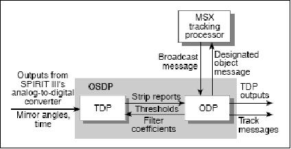
The TDP parameters are fed back from the object-dependent processor (ODP) to improve the signal processing performance. The TDP performs gamma (spike) event circumvention, detector responsivity correction, background subtraction, time delay and integration (TDI), matched filtering, and thresholding. The gamma pulses (spike events) are caused by such phenomena as cosmic ray and proton collisions with the FPA. The process of TDI involves boosting object signal-to-noise ratio (SNR) by coherently adding the outputs of detectors aligned in the scan direction of the sensor. Using the known scan rate, and assuming that object inertial motion is negligible, the data from each detector are stored in a TDI chain for the time delay required to cause each detector to observe the same spatial position.
The ODP is capable of initiating and maintaining tracks on objects in the sensor's field of view. The availability of these tracks gives rise to a number of spin-off functional enhancements, such as (1) feedback of object velocity estimates to correct for velocity distortions in array correlation and matched filtering; (2) windowing, a convenient and computationally efficient form of scan-to-scan correlation; and (3) designated object tracking, where the MSX tracking processor provides (in the broadcast message) a start-up state vector for an object to be tracked.
The TDP-ODP interface and the manner in which the TDP passes thresholded data to the ODP are key to the OSDP design. The TDP hands off matched filter threshold exceedances to the ODP in groups called strip reports, constructed in a manner that maintains the integrity of clumps extending across many pixels. This function is called clump processing.
MSX Ground Segment
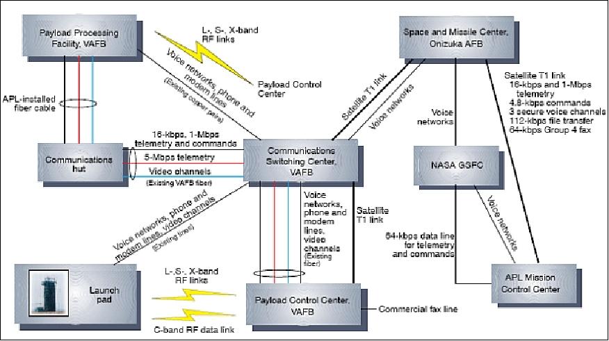
The MSX spacecraft is operated by APL; its S-band is also monitored by AFSCN (Air Force Satellite Control Network). APL also receives the prime science data and provides processing and archiving for all data.
Communications associated with ground operations encompassed a variety of networks that connected the spacecraft to the PCC (Payload Control Center) at a specific test site; to the Command Center at the Air Materiel Command's Detachment 2/Space and Missile Center, Onizuka AFB, CA; or to the MCC (Mission Control Center) at APL. 37)
References
1) "Midcourse Space Experiment: Overview," Johns Hopkins APL Technical Digest, Vol. 17, No 1, January-March 1996, URL: http://www.jhuapl.edu/techdigest/TD/td1701/index.htm
2) John D. Mill, Bruce D. Guilmain, "The MSX Mission Objectives," Johns Hopkins APL Technical Digest, Vol. 17, No 1, January-March 1996, pp. 4-10, URL: http://www.jhuapl.edu/techdigest/TD/td1701/mill.pdf
3) Richard K. Huebschman, "The MSX Spacecraft System Design," Johns Hopkins APL Technical Digest, Vol. 17, No 1, 1996, pp. 41-48, URL: http://www.jhuapl.edu/techdigest/TD/td1701/huebsch.pdf
4) John D. Mill, R. R. O'Neil, S. Price, G. J. Romick, O. M. Uy, et al., "Midcourse Space Experiment: Introduction to the Spacecraft, Instruments, and Scientific Objectives," Journal of Spacecraft and Rockets, Vol. 31, No. 5, September-October 1994, pp. 900-907
5) L. J. Paxton, C.-I. Meng, D. E. Anderson, G. J. Romick, "MSX - A Multiuse Space Experiment," Johns Hopkins APL Technical Digest, Vol. 17, No 1, January-March 1996, pp. 19-34, URL: http://www.jhuapl.edu/techdigest/TD/td1701/paxton.pdf
6) C. Thompson Pardoe, "Keeping the MSX on Track," Johns Hopkins APL Technical Digest, Vol. 17, No 1, 1996, pp. 35-40, URL: http://www.jhuapl.edu/techdigest/TD/td1701/pardoe.pdf
7) "Midcourse Space Experiment (MSX)," DoD/MDA (Missile Defense Agency), Sept. 23, 2015, URL: http://www.mda.mil/news/gallery_msx.html
8) W. E. Skullney, H. M. Kreitz, Jr., M. J. Harold, S. R. Vernon, T. M. Betenbaugh, T. J. Hartka, D. F. Persons, E. D. Schaefer, "Structural Design of the MSX Spacecraft," Johns Hopkins APL Technical Digest, Vol. 17, No 1, January-March 1996, pp. 59-76, URL:http://www.jhuapl.edu/techdigest/TD/td1701/skullney.pdf
9) July A. Krein, Douglas S. Mehoke, "The MSX Thermal Design," Johns Hopkins APL Technical Digest, Vol. 17, No 1, January-March 1996, pp. 49-58, URL: http://www.jhuapl.edu/techdigest/TD/td1701/krein.pdf
10) Paul E. Panneton, Jason E. Jenkins, "The MSX Spacecraft Power Subsystem," Johns Hopkins APL Technical Digest, Vol. 17, No 1, January-March 1996, pp. 77-87, URL: http://www.jhuapl.edu/techdigest/TD/td1701/panneton.pdf
11) D. D. Stott, R. K. Burek, P. Eisenreich, J. E. Kroutil, P. D. Schwartz, G. F. Sweitzer, "The MSX Command and Data Handling System," Johns Hopkins APL Technical Digest, Vol. 17, No 1, January-March 1996, pp. 143-151, URL: http://citeseerx.ist.psu.edu/viewdoc/download?doi=10.1.1.2.9021&rep=rep1&type=pdf
12) L. J. Frank, C. B. Hersman, S. P. Williams, R. F. Conde, "The MSX Tracking, Attitude, and UVISI Processors," Johns Hopkins APL Technical Digest, Vol. 17, No 2, 1996, pp. 137 -142, URL: http://techdigest.jhuapl.edu/TD/td1702/frank.pdf
13) Kristi Marren, "APL-Operated Midcourse Space Experiment Ends," Spacedaily, July 22, 2008, URL: http://www.spacemart.com/reports/APL_Operated_Midcourse_Space_Experiment_Ends_999.html
14) Joseph Scott Stuart, Andrew J. Wiseman, Jayant Sharma, "Space-Based Visible End of Life Experiments," 2008, URL: http://www.amostech.com/TechnicalPapers/2008/SSA_and_SSA_Architecture/Stuart.pdf
15) Michael Norkus, Robert F. Baker, Robert E. Erlandson, "Evolving Operations and Decommissioning of the Midcourse Space Experiment Spacecraft," JHU/APL Technical Digest, Vol. 29, No 3, 2010, pp. 218-225, URL: http://www.jhuapl.edu/techdigest/TD/td2903/Norkus.pdf
16) Thomas E. Strikwerda, Michael Norkus, Richard D. Reinders, "MSX - Maintaining Productivity with an Aging G&C System," Proceedings of the 32nd AAS Guidance and Control Conference, Breckenridge, CO, USA, Jan. 31.- Feb. 4, 2009, AAS - 09-031
17) P. Campbell, "MSX Satellite Celebrates a Decade in Space," URL: http://www.jhuapl.edu/newscenter/stories/st060724.asp
18) "Air Force Space Command Celebrates MSX 10th Anniversary," Spacedaily, April 21, 2006, URL: http://www.spacedaily.com/reports/Air_Force_Space_Command_Celebrates_MSX
_10th_Anniversary.html
19) Jayant Sharma, Grant H. Stokes, Curt von Braun, George Zollinger, Andrew J. Wiseman, "Toward Operational Space-Based Space Surveillance," Lincoln Laboratory Journal, Vol. 13, No 2, 2002, URL: http://citeseerx.ist.psu.edu/viewdoc/download?doi=10.1.1.66.6626&rep=rep1&type=pdf
20) J. F. Carbary, D. Morrison, G. J. Romick, J.-H. Yee, "Spectrum of a Leonid meteor from 110 to 860 nm," Advances in Space Research, Volume 33, Issue 9, 2004, pp. 1455-1458
21) J.-H. Yeh, et al., "Atmospheric remote sensing using a combined extinctive and refractive stellar occultation technique, Overview and proof-of-concept observations," Journal of Geophysical Research, Vol. 107, D14, 2002, p.4213
22) R. J. Vervack, Jr., J.-H. Yee, R. DeMajistre, W. H. Swartz, "Intercomparison of MSX/UVISI-derived ozone and temperature profiles with ground-based, SAGE II, HALOE, and POAM III data," URL: http://www-imk.fzk.de/asf/stratozon/qos2004/cd/files/289.doc
23) A. T. Stair, Jr., "MSX Design Parameters Driven by Targets and Backgrounds," Johns Hopkins APL Technical Digest, Vol. 17, No 1, January-March 1996, pp. 11-18, URL: http://www.jhuapl.edu/techdigest/TD/td1701/stair.pdf
24) J. F. Carbary, E. H. Darlington, K. Heffernan, T. J. Harris, C. I. Meng, M. J. Mayr, P. J. McEvaddy, K. Peacock, "Aerial Surveillance Sensing Including Obscured and Underground Object Detection," Proceedings of SPIE, April 4-6, 1994, Orlando Florida, Volume 2217
25) Brent Y. Bartschi, David E. Morse, Tom L. Woolston, "The Spatial Infrared Imaging Telescope III," Johns Hopkins APL Technical Digest, Vol. 17, No 2, 1996, pp. 215-225, URL: http://techdigest.jhuapl.edu/TD/td1702/bartschi.pdf
26) K. J. Heffernan, J. E. Heiss, J. D. Boldt, E. Hugo Darlington, K. Peacock, T. J. Harris, M. J. Mayr, "The UVISI Instrument," Johns Hopkins APL Technical Digest, Vol. 17, No 2, 1996, pp. 198-214, URL: http://techdigest.jhuapl.edu/TD/td1702/hefernan.pdf
27) Ronald J. Vervack Jr., Jeng-Hwa Yee, William H. Swartz, Robert DeMajistre, Larry J. Paxton, "The MSX/UVISI Stellar Occultation Experiments: Proof-of-Concept Demonstration of a New Approach to Remote Sensing of Earth's Atmosphere," JHU/APL Technical Digest, Vol. 32, No 5, 2014, pp: 803-821, URL: http://techdigest.jhuapl.edu/TD/td3205/32_05-Vervack.pdf
28) P. B. Hays, R. G. Roble, "Stellar Spectra and Atmospheric Composition," Journal of Atmospheric Sciences, Vol. 25, No 6, pp: 1141–1153, 1968
29) J.-H. Yee, R. J. Jr. Vervack, R. DeMajistre, F. Morgan, J. F. Carbary, et al., "Atmospheric Remote Sensing Using a Combined Extinctive and Refractive Stellar Occultation Technique: 1. Overview and Proof-of-Concept Observations," Journal of Geophysical Research, Vol. 107(D14), ACH 15-1–ACH 15-13 , 2002
30) R. DeMajistre, J.-H. Yee, "Atmospheric Remote Sensing Using a Combined Extinctive and Refractive Stellar Occultation Technique: 2. Inversion Method for Extinction Measurements," Journal of Geophysical Research, Vol. 107(D15), ACH 6-1–ACH 6-18, 2002
31) R. J. Jr. Vervack, J.-H. Yee, J. F. Carbary, F. Morgan, "Atmospheric Remote Sensing Using a Combined Extinctive and Refractive Stellar Occultation Technique: 3. Inversion Method for Refraction Measurements," Journal of Geophysical Research, Vol. 107(D15), ACH 7-1–ACH 7-19, 2002
32) David C. Harrison, Joseph C. Chow, "The Space-Based Visible Sensor," Johns Hopkins APL Technical Digest, Vol. 17, No 2, 1996, pp. 226-236, URL: http://techdigest.jhuapl.edu/TD/td1702/harrison.pdf
33) Grant H. Stokes, Curt von Braun, Ramaswamy Sridharan, David Harrison, Jayant Sharma, "The Space-Based Visible Program," Lincoln Laboratory Journal, Vol. 11, No 2, 1998, pp. 205-238, URL: http://citeseerx.ist.psu.edu/viewdoc/download?doi=10.1.1.70.8068&rep=rep1&type=pdf
34) Joan H. Cranmer, Jack T. Sanders, Jr.. Jeffrey C. Lesho, O. Manuel Uy, "Contamination Control for the MSX: An Overview," Johns Hopkins APL Technical Digest, Vol. 17, No 1, 1996, pp. 88-101, URL: http://www.jhuapl.edu/techdigest/TD/td1701/cranmer.pdf
35) O. M. Oy, "Midcourse Space Experiments (MSX) Contamination Results," Space & Environmental Flight Experiments Workshop, Huntsville, AL, June 23-25, 1998
36) C. G. Pfeiffer, B. L. Masson, "Technology Demonstration by the Onboard Signal and Data Processor," Johns Hopkins APL Technical Digest, Vol. 17, No 2, 1996, pp. 237-245, URL: http://techdigest.jhuapl.edu/TD/td1702/pfeiffer.pdf
37) J. F. Smola, M. H. Barbagallo, J. H. Cranmer, C. C. DeBoy, M. J. Harold, J. A. Krein, H. M. Kreitz, Jr., A. C. Sadilek, H. K. Utterback, "MSX Ground Operations," Johns Hopkins APL Technical Digest, Vol. 17, No 2, 1996, pp. 173-188, URL: http://citeseerx.ist.psu.edu/viewdoc/download;jsessionid=A6A2773C3E103155D09DB01879516C60?doi=10.1.1.5.3344&rep=rep1&type=pdf
38) Robert D. Nordeen, Valerie B. Barnes, Andrew C. Good, Raymond J. Harvey, "The MSX Flight Operations System," Johns Hopkins APL Technical Digest, Vol. 17, No 1, January-March 1996, pp. 102-116, URL: http://www.jhuapl.edu/techdigest/TD/td1701/nordeen.pdf
The information compiled and edited in this article was provided by Herbert J. Kramer from his documentation of: "Observation of the Earth and Its Environment: Survey of Missions and Sensors" (Springer Verlag) as well as many other sources after the publication of the 4th edition in 2002. - Comments and corrections to this article are always welcome for further updates (eoportal@symbios.space).
Overview Spacecraft Launch Mission Status Sensor Complement MSX Ground Segment References Back to top