Landsat-7
EO
Atmosphere
Ocean
Cloud type, amount and cloud top temperature
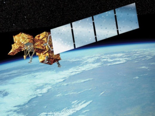
Launched in April 1999, Landsat-7 is part of NASA’s Earth Science Enterprise (ESE) program, a joint venture by NASA and USGS (United States Geological Survey). As a successor of Landsat-6, which failed upon launch, the objective of Landsat-7 is to enhance the medium-resolution multispectral imagery of Earth’s continental surfaces provided by previous Landsat satellites. Although it had an initial design life of seven years, Landsat-7 remains operational as of July 2022 and was joined by Landsat-8 in February 2013, and Landsat-9 in September 2021.
Quick facts
Overview
| Mission type | EO |
| Agency | NASA, USGS |
| Mission status | Operational (extended) |
| Launch date | 15 Apr 1999 |
| Measurement domain | Atmosphere, Ocean, Land, Snow & Ice |
| Measurement category | Cloud type, amount and cloud top temperature, Ocean colour/biology, Multi-purpose imagery (ocean), Radiation budget, Multi-purpose imagery (land), Surface temperature (land), Vegetation, Albedo and reflectance, Sea ice cover, edge and thickness, Snow cover, edge and depth, Inland Waters |
| Measurement detailed | Ocean imagery and water leaving spectral radiance, Ocean chlorophyll concentration, Cloud cover, Cloud imagery, Land surface imagery, Fire temperature, Vegetation type, Fire fractional cover, Earth surface albedo, Short-wave Earth surface bi-directional reflectance, Leaf Area Index (LAI), Land cover, Land surface temperature, Sea-ice cover, Snow cover, Normalized Differential Vegetation Index (NDVI), Iceberg fractional cover, Fraction of Absorbed PAR (FAPAR), Glacier motion, Glacier cover, Sea-ice surface temperature, Above Ground Biomass (AGB), Active Fire Detection, Long-wave Earth surface emissivity, Permafrost, Evapotranspiration, Cloud mask, Surface Water Extent, Mineral Type |
| Instruments | ETM+ |
| Instrument type | Imaging multi-spectral radiometers (vis/IR) |
| CEOS EO Handbook | See Landsat-7 summary |
Related Resources
Summary
Mission Capabilities
Landsat-7 features the Enhanced Thermal Mapper Plus (ETM+) developed by Raytheon SBRS (Santa Barbara Remote Sensing) which builds upon the Thermal Mapper (TM) onboard Landsat-4 & -5. ETM+ is a whiskbroom scanning radiometer capable of imaging in eight distinct bands including four visible and near-infrared (VNIR), two short wave infrared (SWIR), one thermal infrared (TIR) and one panchromatic (PAN) band. The addition of the PAN band, improved resolution and two 8-bit “gain” ranges in ETM+ have led to Landsat data progressing into use for global scale studies. Data acquired using ETM+ has applications in land cover/change monitoring, agricultural forecasting, disaster response, urban planning, land and water resource management, and ecosystem monitoring.
Performance Specifications
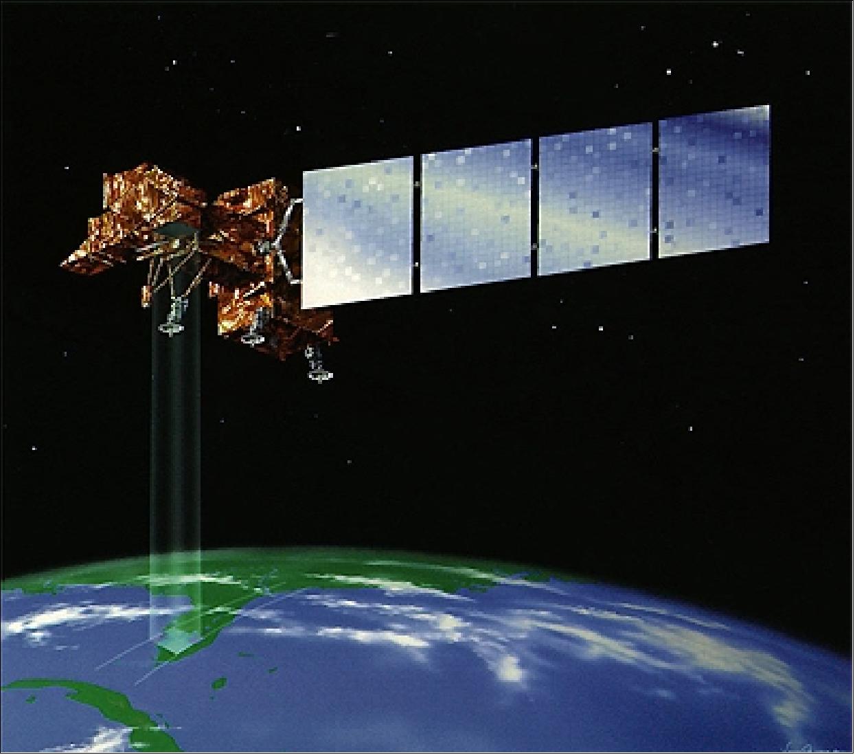
ETM+ images with a spatial resolution of 15 m for the PAN band, 30 m for VNIR/SWIR bands and 60 m for the TIR band, each covering a swath of 185 km. The scanner contains two focal planes and detector line arrays oriented in the long-track direction. This arrangement provides parallel coverage of 480 m along-track in one scan sweep (cross-track direction). The wide along-track coverage permits sufficient integration time for all cells in each scan sweep.
Landsat-7 undergoes a sun-synchronous polar orbit at an altitude of 705 km with an inclination of 98.2°. The nominal descending equator crossing time is at 1000-1015, with a period of 99 minutes and repeat coverage of 16 days.
Space and Hardware Components
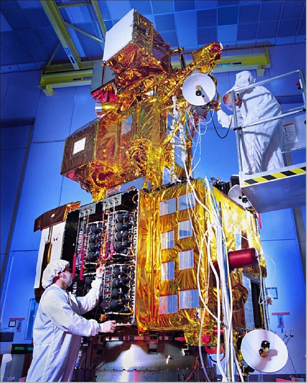
Built by LMMS (Lockheed Martin Missiles and Space), the Landsat-7 spacecraft uses a very similar design to its predecessor, Landsat-6. With a mass of 2200 kg, the satellite features the three-axis stabilised Landsat-6 bus with an onboard recorder in solid state memory. Attitude control is provided by four reaction wheels and two torque rods, sensed with a static Earth sensor, two magnetometers and gyroscopes. The satellite is powered by a four-panel silicon cell solar array and two nickel hydrogen batteries. Orbit control and backup momentum is provided through a blow-down monopropellant hydrazine system with a single tank containing 122 kg of hydrazine.
In May 2003 the Scan Line Corrector (SLC) on ETM+ failed. The function of the SLC was to compensate for the forward motion of the satellite during data acquisition, thus as a consequence of its failure, individual image scans overlap and leave large physical gaps near the edge of each picture. Overall, approximately 30% of the total image is missing in each downlinked picture.
Landsat-7
Spacecraft Launch Mission Status Ground Segment References
The Landsat-7 satellite is part of NASA's ESE (Earth Science Enterprise) program, a joint venture of NASA and USGS (United States Geological Survey). The overall mission objective is to extend and improve upon the long-term record of medium-resolution multispectral imagery of the Earth's continental surfaces provided by the earlier Landsat satellites. 1)
Following the loss of Landsat-6 during launch in 1993, Landsat-7 was placed on a fast track for launch in 1998, but was ultimately launched on 15 April 1999 (a one-year delay resulted from having to replace some faulty electronics inside the ETM+ sensor).
Spacecraft
The S/C and payload were developed under NASA/GSFC management/procurement responsibility (Landsat Project Scientist: D. Williams). The LS-7 satellite was built by LMMS (Lockheed Martin Missiles and Space) at the facility in Valley Forge, PA. The S/C features the Landsat-6 bus; an onboard recorder in solid state memory (378 Gbit capacity to capture data beyond the range of ground receiving stations, recording rates of 150 Mbit/s, playback with 300 Mbit/s), and a single observation instrument: ETM+. 2) 3)
The Landsat-7 spacecraft is very similar in design to the Landsat-6 satellite. It features three-axis stabilization with a pointing capability of 180 arcsec (3σ) and a pointing knowledge of 45 arcsec (1σ). Attitude control is provided with four reaction wheels and two torque rods, attitude is sensed with a static Earth sensor, 2 magnetometers and gyros. Orbit control and backup momentum unloading is provided through a blow-down monopropellant hydrazine system with a single tank containing 122 kg of hydrazine.
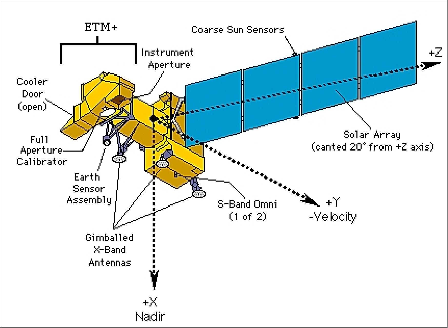
S/C mass = 2200 kg, dimensions: 4.3 m in length and 2.8 m in diameter, power = 1550 W [about 1000 W average, provided by a silicon cell solar array (4 panels each of size 1.88 m x 2.26 m) and two nickel hydrogen batteries each of 50 Ahr capacity]. S/C design life = 7 years.
The onboard processor performs autonomously executed functions for wideband communications, electrical power management, and satellite control. These include attitude control, redundancy management, antenna steering, battery management, solar array pointing maintenance, thermal profile maintenance, and stored command execution.
RF communications: All data communication is CCSDS compliant. An onboard SSR (Solid State Recorder) is used to capture wideband data from the ETM+ (storage capacity of 378 Gbit, equivalent for about 100 scenes or 42 minutes of instrument data).
• S-band (2 omni-directional antennas), 5 W, for TT&C data with real-time telemetry data rates of 1.2 kbit/s and 4.8 kbit/s, and 256 kbit/s of playback data, 2 kbit/s of command data. S-band frequencies of 2106.4 MHz (uplink) and 2287.5 MHz (downlink). The zenith antenna is used for TDRS (Tracking Data and Relay Satellite) communications; the nadir antenna is used for Landsat Ground Network (LGN) communications. Each antenna provides essentially hemispherical coverage.
• X-band (3 steerable antennas), 3.5 W; each antenna transmits data on two channels, with each channel carrying 75 Mbit/s (total of 150 Mbit/s per antenna); up to three separate links are supported. X-band frequencies: 8082.5 MHz, 8212.5 MHz, 8342.5 MHz. The downlink beam width of each antenna is 1.2º.
Ground sites exist at Sioux Falls, South Dakota (Landsat Ground Station, or LGS), Poker Flat, Alaska (Alaska Ground Station, or AGS), Wallops Virginia (WPS), and Svalbard, Norway (SGS). All ground sites are equipped with 11 meter antennas. AGS, SGS, and LGS are capable of receiving both S-band (TT&C) at a downlink rate of 4 kbit/s and X-band (payload) data simultaneously.
Launch
Launch: A launch of Landsat-7 took place on a Delta 2 vehicle from VAFB, CA on April 15, 1999.
Orbit: Sun-synchronous polar orbit (AM orbit), altitude = 705 km, inclination = 98.2º, period = 99 minutes, repeat coverage = 16 days, the nominal descending equator crossing time is at 10:00 to 10:15 hours.
The ground track is referenced to WRS (Worldwide Reference System) with a repeat accuracy of ±5 km. The WRS indexes orbits (paths) and scene centers (rows) into a global grid system (daytime and night time) comprising 233 paths by 248 rows. 4)
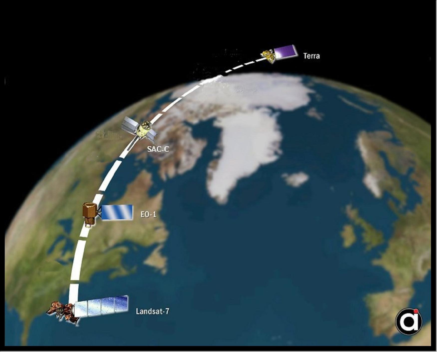
As of early 2001 Landsat-7 is flying in the so-called “morning constellation,” also referred to as morning train with EO-1 (a few minutes apart), SAC-C and Terra. The objective is to compare coincident imagery from the ETM+ and ALI instruments. The “paired scene” images are used to evaluate the performance of ALI. In fact, the EO-1 and SAC-C spacecraft joined the constellation already on Nov. 21, 2000. The overall objective is to obtain synergistic effects for data interpretation and analysis.
Sensor Complement
ETM+ (Enhanced Thematic Mapper Plus)
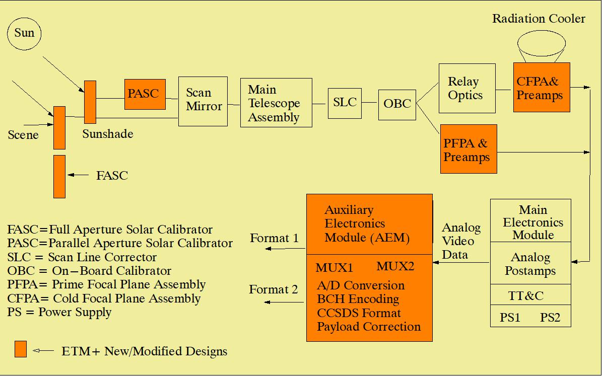
ETM+ was built by Raytheon SBRS (Santa Barbara Remote Sensing), Goleta, CA. ETM+ is an 8-band whiskbroom scanning radiometer consisting of:
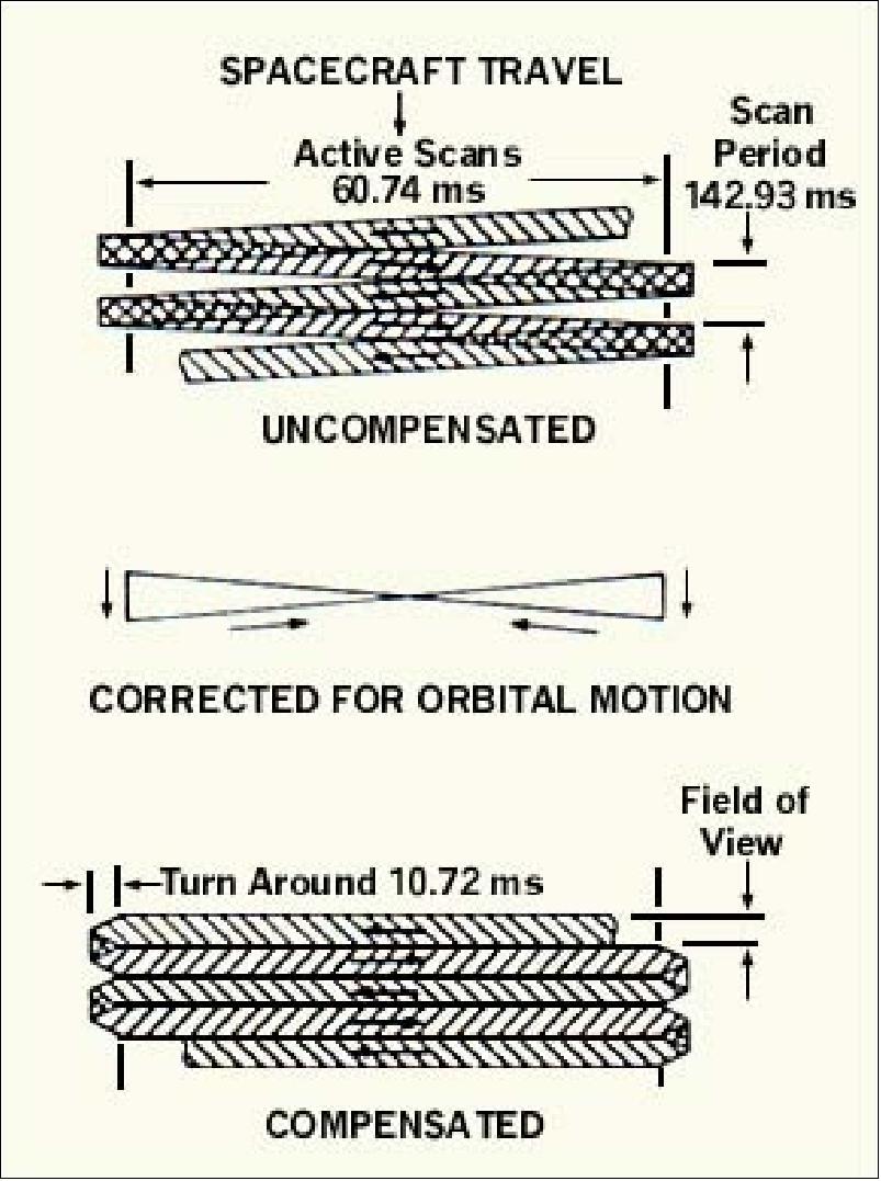
• A primary mirror that sweeps side-to-side (cross-track) to produce forward and revers image scans, and
• A scan line corrector (SLC) mirror assembly that sweeps forward-to-aft to compensate for the forward motion of the spacecraft during integration time. The motion of these mirrors deviates from an ideal line profile, introducing along- and cross-track geometric distortions that require compensation.
The principal functional differences between the ETM and the former TM series are the addition of a 15 m resolution panchromatic band and two 8-bit “gain” ranges. The ETM+ adds a 60 m resolution thermal band, replacing the 120 m band on ETM/TM (band No. 6). Design life = 7 years. 5)
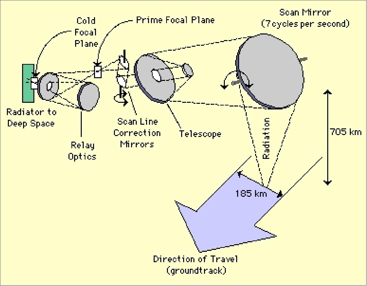
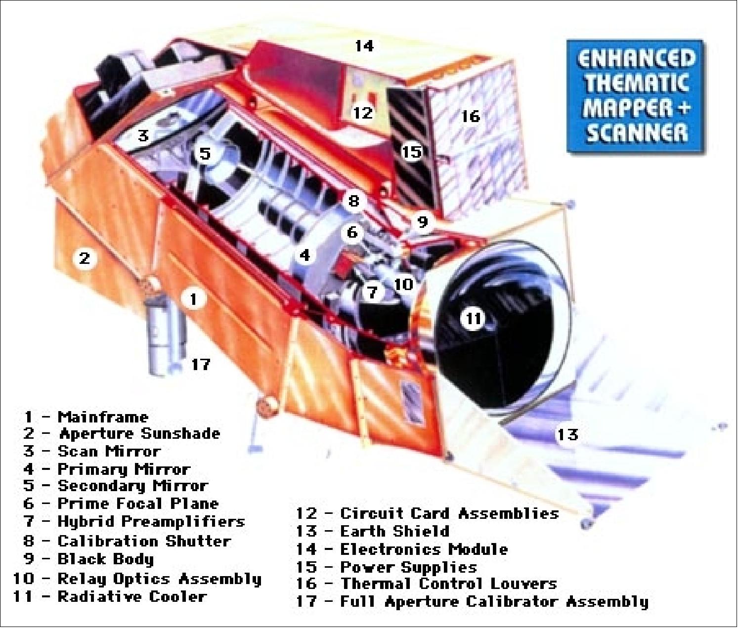
The Scan Mirror Assembly (SMA) provides the cross-track scanning motion to develop the 185 km long scene swath. The SMA consists of a flat mirror supported by flex pivots on each side (which have compensators to equalize pivot reaction torque), a torquer, a scan angle monitor (SAM), 2 leaf spring bumpers and scan mirror electronics (SME). The bi-directional SMA sweeps the detector's line of sight in west-to-east and east-to-west directions in cross-track direction, while the spacecraft's orbital path provides the north-south motion.
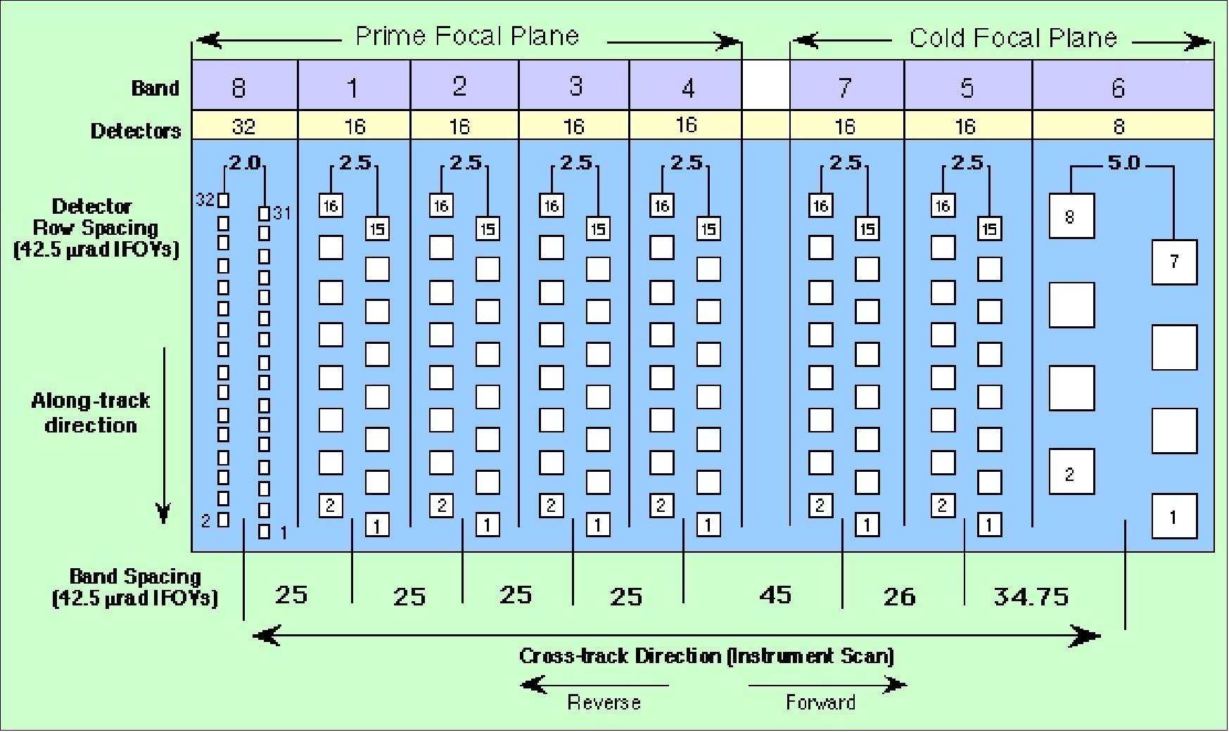
The ETM+ scanner contains 2 focal planes that collect, filter, and detect the scene radiation in a swath, 185 km wide. The primary focal plane consists of optical filters, detectors, and preamplifiers for 5 of the 8 ETM+ spectral bands (bands 1-4, 8). The second focal plane is the cold focal plane which includes the optical filters, infrared detectors, and input stages for ETM+ spectral bands 5,6, and 7. The temperature of the cold focal plane is maintained at 91 K using a radiative cooler. The detector line arrays (16 for VNIR bands, 32 for PAN, and 8 detectors for TIR) of the whiskbroom scanner are oriented in the along-track direction. This arrangement provides a parallel coverage of 480 m along-track in one scan sweep (cross-track direction). The wide along-track coverage permits sufficient integration time for all cells in each scan sweep.
Band No. | Wavelength (µm) | Detectors | IFOV (µrad) | GSD (m) | SNR (at min signal radiance) |
8 PAN | 0.52 - 0.90 | SiPD (32) | 18.5 x 21.3 | 13 x 15 | 15 |
1 VIS | 0.45 - 0.52 | SiPD (16) | 42.5 | 30 x 30 | 32 |
2 VIS | 0.53 - 0.61 | SiPD (16) | 42.5 | 30 | 35 |
3 VNIR | 0.63 - 0.69 | SiPD (16) | 42.5 | 30 | 26 |
4 VNIR | 0.78 - 0.90 | SiPD (16) | 42.5 | 30 | 32 |
5 SWIR | 1.55 - 1.75 | InSb (16) | 42.5 | 30 | 25 |
7 SWIR | 2.09 - 2.35 | InSb (16) | 42.5 | 30 | 17 |
6 TIR | 10.4 - 12.5 | HgCdTe (8) | 85.2 | 60 | 0.5 K |
The ETM+ also includes a number of radiometric enhancements to achieve an absolute radiometric uncertainty of <5% (bands 1-4). Two new calibration devices were added: FAC (Full Aperture Calibrator), and PAC (Partial Aperture Calibrator). ETM+ uses three independent onboard calibration systems (plus preflight calibration), representing a significant step forward in absolute radiometric calibration accuracy. 6) 7)
• A full-aperture solar diffuser (FASC) on the inner surface of the aperture door that illuminates the focal planes with diffusely reflected solar energy when commanded into position
• A partial-aperture solar reflector (PASC) that illuminates the focal planes with attenuated solar energy, once per orbit
• Internal calibrator (IC). Calibration lamps that project calibrated energy onto the focal planes via the main calibration shutter, once per scan, during the scan mirror turnaround.
From the initiation of the LS-7 system, greater attention was paid toward the long-term characterization and calibration of the data than for earlier LS missions. In particular, an IAS (Image Assessment System) was incorporated into the ground processing system. The objective of IAS is to characterize and calibrate the instrument data over the life of the mission. 8) 9) 10) 11) 12)
Scanning method | Bidirectional cross-track, scan frequency = 7 Hz |
Scan period | 142.9 ms, (scan frequency of 6.99 Hz) |
Swath width | 185 km (15º FOV from 705 km orbit) |
Telescope | 40.6 cm aperture diameter, Ritchey-Chretien configuration with a primary and secondary mirror and baffles; mirror material: ULE (Ultra Low Expansion) glass |
Effective focal length | 243.8 cm, (f/6.0) |
Instrument size | Scanner assembly: 1.5 m x 0.7 m x 2.5 m |
Instrument mass | Scanner assembly: 298 kg, AEM = 103 kg, cable harness = 20 kg |
Power | 590 W |
Data quantization | 9 bit A/D conversion, 8 bit/pixel transmitted (2 gain states) |
Data rate | 150 Mbit/s (2 x 75) by each of three directional X-band antennas, CCSDS format |
Cross calibration was performed between ETM+ and ALI [(Advanced Land Imager) on the EO-1 (Earth Observing-1) mission] image pairs using two approaches. One approach was based on image statistics of large common areas between the image pairs. The other approach was based on vicarious calibration that compares the measured radiance obtained from the sensor to the predicted at-sensor radiance using the surface measurements propagated to the sensor via radiative transfer code. 13) 14) 15)
Landsat sensor | MSS | TM | ETM | ETM+ |
Spectral bands (all bands in µm) | 1) 0.5 - 0.6 | 1) 0.45 - 0.52 VNIR | P) 0.52 - 0.90 VNIR | P) 0.52 - 0.90 VNIR |
Swath width | 185 km | 185 km | 185 km | 185 km |
Spatial | 80 m | 30 m VNIR/SWIR | 15 m PAN, 30 m VNIR/SWIR, 120 TIR | 15 m PAN |
Radiometric resolution | 6 bit | 8 bit | 9 bit (8 bit transmitted) | 9 bit (8 bit transmitted) |
Band-to-band registration |
| 0.2 pixel (90%) | 0.2 pixel (90%) | 0.2 pixel (90%) |
Geodetic accuracy without ground control |
| 500 m (90%) | 1000 m (90%) | 400 m (90%) |
Data rate | 15 Mbit/s | 85 Mbit/s | 2 x 85 Mbit/s | 2 x 75 Mbit/s |
Instrument mass | 64 kg | 258 kg | 288 kg scanner, plus 81 kg AEM | 318 kg scanner, plus |
Average power | 50 W | 332 W | 490 W | 590 W |
Telescope aperture | 23 cm | 40.6 cm | 40.6 cm | 40.6 cm |
Sensor Status
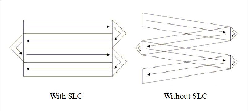
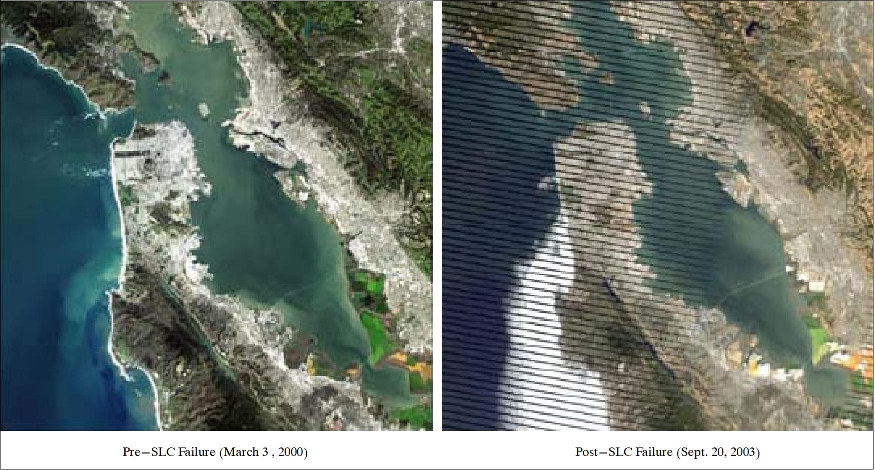
The SLC (Scan Line Corrector) on the ETM+ instrument failed on May 31, 2003. The SLC function is to compensate for the forward motion of the satellite during data acquisition. As a consequence of this operational anomaly, individual image scans overlap and also leave large physical gaps near the edge of each picture. Only portions of the image near the center are left completely unfettered and valid. Overall, about 30 percent of the total image is missing in each downlinked picture.
Spacecraft controllers immediately suspended normal LS-7 operations and limited activity to just spacecraft housekeeping and operations related to the anomaly investigation and recovery effort. However, subsequent efforts to recover the SLC were not successful and the problem appears to be permanent. Without an operating SLC, the ETM+ line of sight now traces a zig-zag pattern along the satellite ground track (Figure 10). The resulting gaps in coverage range from none at the center of the scan to 14 pixels at the extreme edges of the scan.
As of Sept. 16, 2003, LS-7 has resumed its normal Long Term Acquisition Plan (LTAP) scheduling of approximately 250 scenes per day, and all data will now be acquired in SLC-off mode. ETM+ is still capable of acquiring useful image data with the SLC turned off, particularly within the central portion of any given scene.
As of Oct. 2003, the USGS/NASA Landsat team is trying to develop means to compensate for the SLC malfunction, with image processing methods and acquisition strategies to exploit the remaining observation capability of the LS-7 system. The team is refining gap-filling techniques that merge data from multiple acquisitions. They are also developing modifications to the LS-7 acquisition scheme to acquire two or more clear scenes as near in time as possible to facilitate this gap-filling process. These merged images potentially resolve most, if not all, of the missing data problems.
The USGS reinitiated routine collection of ETM+ data with the SLC turned off on July 14, 2003 and began distributing this data in late October 2003. Initially, the USGS offered data products with a fixed maximum interpolation of two pixels in their fully processed data products. Beginning in mid-Feb. 2004, the maximum amount of interpolation became user selectable. Starting in May 2004, USGS began providing the first in a series of data products to help make the SLC-off data more usable. 16) 17) 18)
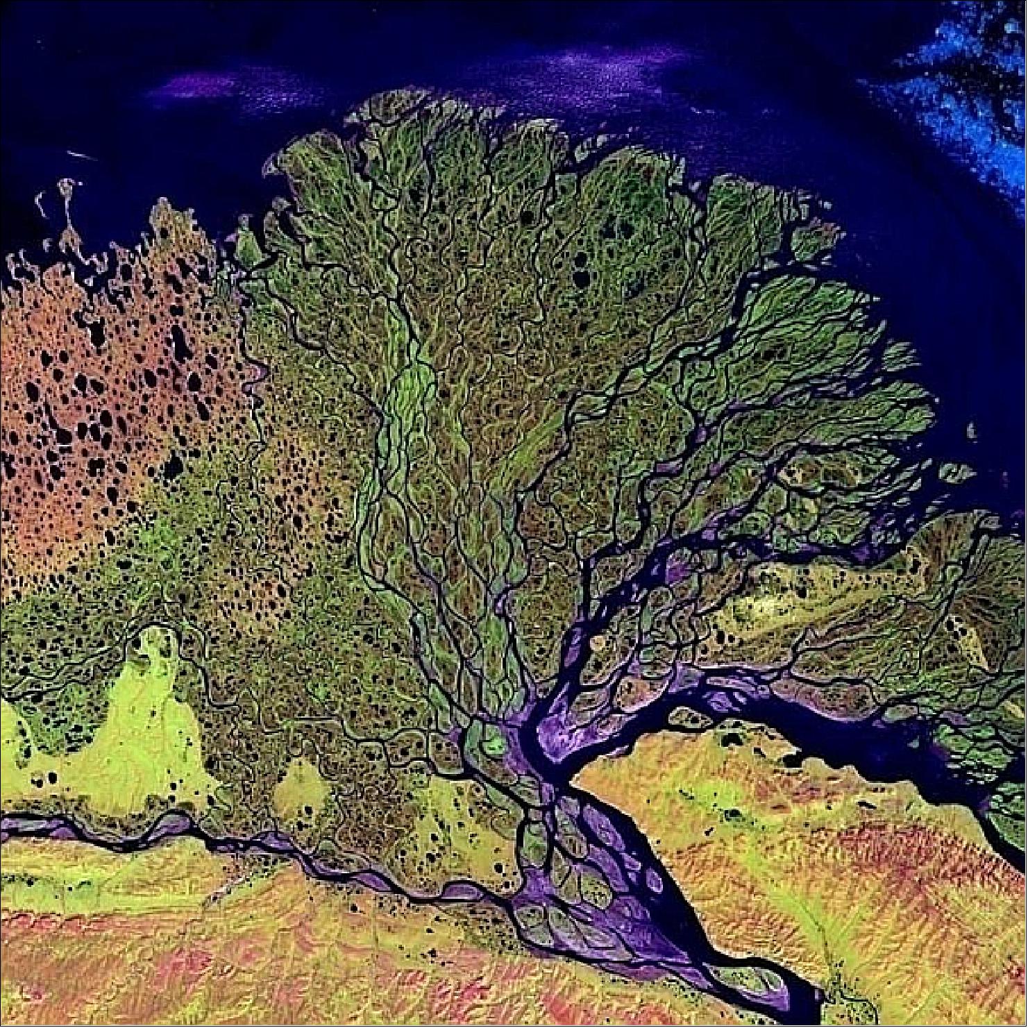
Legend to Figure 12: The Lena river of 4,400 km in length, is one of the largest rivers in the world. The Lena Delta Reserve is the most extensive protected wilderness area in Russia. It is an important refuge and breeding grounds for many species of Siberian wildlife. 20)
Mission Status
• May 5, 2022: Landsat 7 imaging resumed at a lower orbit of 697 km. Data from the L7 extended science mission are currently being released & will all be available by the end of August. 68)
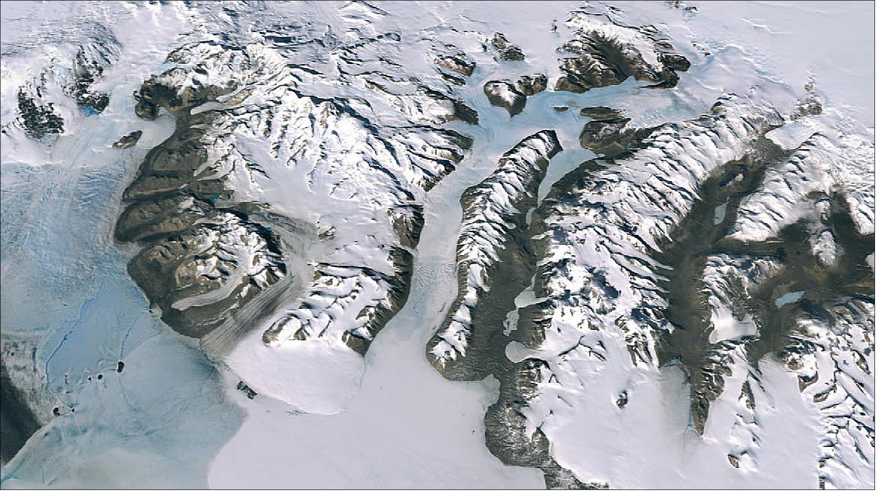
•January 26, 2021: Sverdrup Glacier in northwest Greenland is pretty average. It is a textbook example of the many coastal glaciers around the island that flow into deep fjords. But Sverdrup also represents a large class of Greenland glaciers that are undergoing rapid retreat in response to warm ocean water. 21)
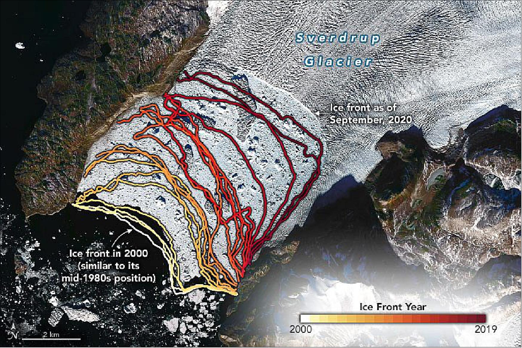
- The position in 2000 was similar to the mid-1980s, indicating that there had been a period of stability when ocean temperatures were cool. Then, between 1998 and 2007, waters around Greenland warmed rapidly—almost 2 degrees Celsius—and the glacier started to thin, flow faster, and retreat.
- “Sverdrup Glacier’s retreat and ice loss was ‘triggered’ by warm water,” said Michael Wood, a postdoctoral researcher at NASA’s Jet Propulsion Laboratory (JPL). “It is one of many deep glaciers that are now in an unstable configuration, and will likely continue to retreat for many years, no matter what the ocean does.”
- To assess how warming ocean water affects coastal glaciers, scientists with the Oceans Melting Greenland (OMG) mission have been studying these marine-terminating glaciers from the air and by ship. In a recent study led by Wood, scientists used these data to show that when it comes to glacier melting, the depth of the fjord matters.
- Glaciers in deep fjords come into contact with more warm ocean water than glaciers in shallow fjords. This hastens undercutting—a process in which a layer of warm, salty water at the bottom of a fjord melts the base of a glacier, causing the ice above to break apart.
- Of the 226 glaciers surveyed, 74 in deep fjords accounted for nearly half of the total ice loss from Greenland between 1992 and 2017. These glaciers exhibited the most undercutting. In contrast, the 51 glaciers that extend into shallow fjords or onto shallow ridges experienced the least undercutting and contributed only 15 percent of the total ice loss.
- “We have known for well over a decade that the warmer ocean plays a major role in the evolution of Greenland glaciers,” said Eric Rignot, OMG deputy principal investigator at JPL. “But for the first time, we have been able to quantify the undercutting effect and demonstrate its dominant impact on the glacier retreat over the past 20 years.”
- These findings suggest that climate models may underestimate glacial ice loss by at least a factor of two if they don’t account for undercutting by a warm ocean.
- The study also lends insight into why many of Greenland’s glaciers never recovered after the abrupt warming of ocean water between 1998 and 2007. Although ocean warming paused between 2008 and 2017, the glaciers had already experienced such extreme undercutting in the previous decade that they continued to retreat at an accelerated rate.
- “When the ocean speaks, the Greenland Ice Sheet listens,” said OMG Principal Investigator Josh Willis, also of JPL. “This gang of 74 glaciers in deep fjords is really feeling the influence of the ocean; it’s discoveries like these that will eventually help us predict how fast the ice will shrink. And that’s a critical tool for both this generation and the next.”
• December 7, 2020: Trees play a vital role in Earth’s carbon and water cycles. They also contribute food, firewood, and other resources important to human activity. But while forests are easy to spot from above, smaller stands of trees have often gone undercounted because they have been harder to detect with the satellite imagers usually available to scientists. 22)
- Now an international team of scientists has used artificial intelligence and commercial satellites to identify an unexpectedly large number of trees spread across arid and semi-arid areas of western Africa. These drylands were previously classified as having little to no tree cover, but new analysis techniques proved otherwise. The findings could help scientists better understand and quantify the role drylands have in the storage and cycling of carbon. 23)
- The research team used the Blue Waters supercomputer at the University of Illinois and an artificial intelligence technique called “deep learning” to map the trees. Led by Martin Brandt of the University of Copenhagen, the team first spent a year examining commercial satellite imagery by eye and identifying 90,000 individual trees in order to build a training dataset for the computer. Ankit Kariryaa of the University of Bremen led the development of the deep learning computer processing.
- Once Brandt and colleagues developed and tested their dataset, Blue Waters—one of the fastest supercomputers in the world—took just a few days to identify nearly 2 billion trees across 1.3 million km2 (500,000 square miles) of sub-Saharan Africa.
- Previous land cover mapping studies of the region relied on satellite imagery with 10– or 30–meter resolution (the distance visible within each pixel). Such studies classified large swaths as grassland or bare soil whenever trees covered less than 20 percent of the land area.

- Brandt’s machine-learning method identified 1.8 billion individual trees standing outside of areas classified as forests. It also measured the crown diameter of each tree. Tree cover was, predictably, higher in areas with more rainfall. “The canopy cover increases from 0.1 percent (0.7 trees per hectare) in hyper-arid areas, through 1.6 percent (9.9 trees per hectare) in arid and 5.6 percent (30.1 trees per hectare) in semi-arid zones, to 13.3 percent (47 trees per hectare) in sub-humid areas,” the researchers wrote in Nature. “Although the overall canopy cover is low, the relatively high density of isolated trees challenges prevailing narratives about dryland desertification and even the desert shows a surprisingly high tree density.”
- Mapping trees outside of forests at this level of detail would take months or years with traditional analysis methods, so the use of very high-resolution imagery and machine learning represents a significant breakthrough. The next steps for the research team include expanding their study area to survey more of Africa and estimating the carbon contained within these trees. “We don’t know much about the role of these dryland areas in the global carbon cycle,” said Brandt. “This research is a step towards filling that knowledge gap.”
- Brandt and colleagues have published their dataset—which includes the location and crown diameter of trees in western Africa—through the Oak Ridge National Laboratory Distributed Active Archive Center (ORNL DAAC). Users can also find it through a NASA Earthdata search.
• August 2019: ”The Living Legacy of Landsat 7: Still Going Strong after 20 Years in Orbit.” 24) 25)
The twentieth anniversary of the launch of Landsat 7 on April 15, 1999, is an opportune time to retrace the history leading to modern Earth science data acquisition and use. This article provides a retrospective, with some insight into why Landsat 7 was a key player in Earth science and related technical endeavors, and how its mission has informed Earth system science to this day. It discusses some of the scientific and technology bases for the Landsat program generally and Landsat 7 specifically, and points out ways in which Landsat 7 crossed organizational boundaries to ensure the best scientific return. Other topics include a significant advance in storing and transmitting data, advances in sensor technology on Landsat 7 and an ongoing mechanical problem with that key sensor.
When Landsat 7 was launched, the ETM+ instrument onboard was the most sophisticated Landsat sensor yet. ETM+ carried a new 15 m panchromatic band and had a refined thermal band with a 60 m spatial resolution (compared to 120 m for Landsats 4 and 5). Landsat 7 also utilized a new solid-state data recorder (SSR)—the first to fly on a civilian mission.
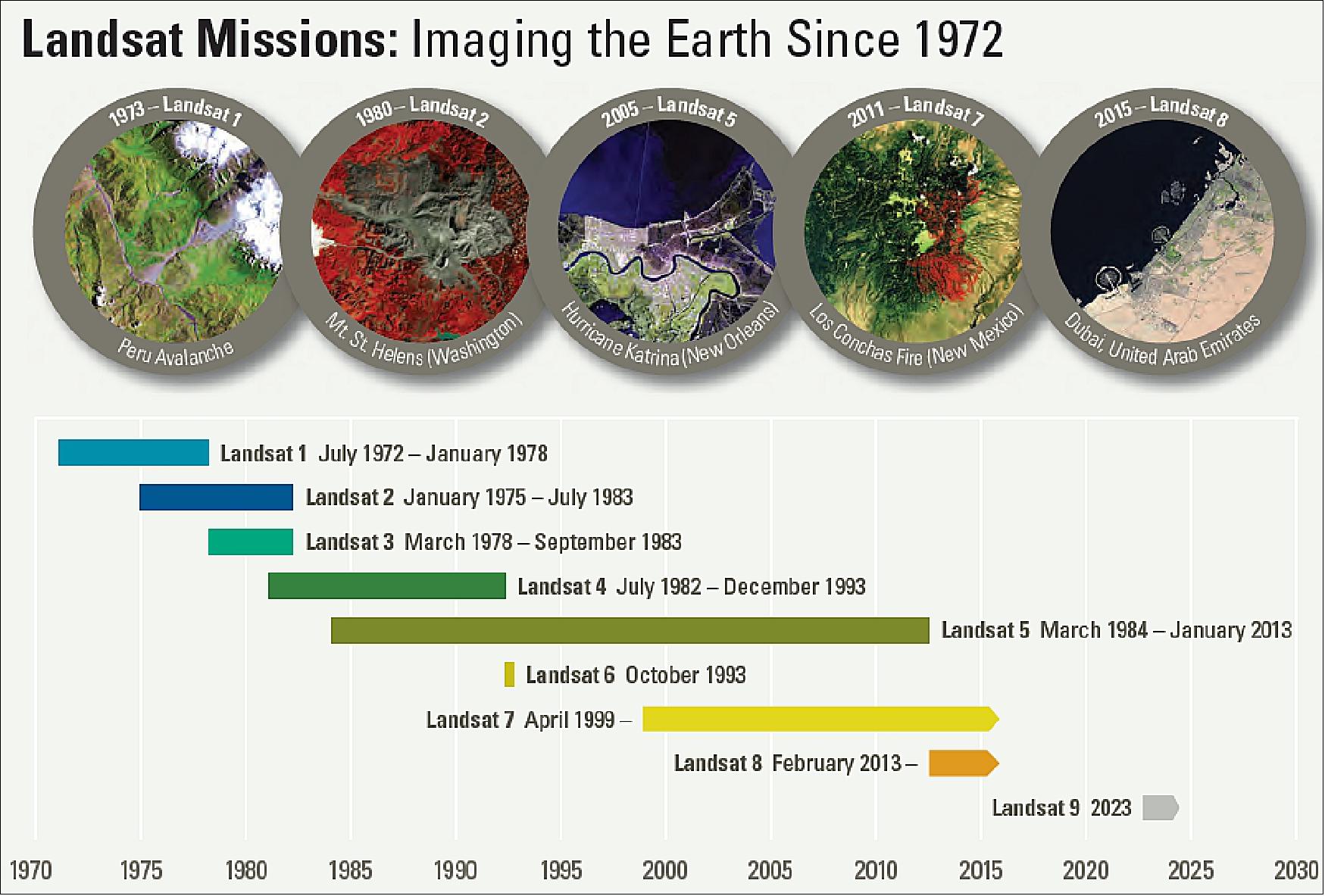
Satellite | Launch Date | Sensor | Resolution (m) and | Communication | Altitude (km) | Repeat Cycle |
Landsat 1 | July 23, 1972 | RBV | 80/VNIR | Direct downlink | 917 | 18 |
Landsat 2 | January 22, 1975 | RBV | 80/VNIR | Direct downlink | 917 | 18 |
Landsat 3 | March 5, 1978 | RBV | 40/PAN | Direct downlink | 917 | 18 |
Landsat 4 | July 16, 1982 | MSS | 80/VNIR | Direct downlink | 705 | 16 |
Landsat 5 | March 1, 1984 | MSS | 80/VNIR | Direct downlink | 705 | 16 |
Landsat 6 | (October 5, 1993) | ETM | 15/PAN | Direct downlink | 705 | 16 |
Landsat 7 | April 15, 1999 | ETM+ | 15/PAN | Direct downlink | 705 | 16 |
Landsat 8 | February 11, 2013 | OLI | 15/PAN, 30/VNIR/SWIR | Direct downlink | 705 | 16 |
Early Success, but with a Long-Term Problem: While the launch and subsequent checkout of Landsat 7 went well, after four flawless years of operation, problems emerged. On May 31, 2003, the Scan Line Corrector (SLC) failed, resulting in lack of data in several narrow wedge-shaped slivers on acquired scenes. The SLC’s role was to compensate for the orbital motion of the platform during forward and return scans to create parallel sweeps across the Earth’s surface; without it, a zig-zag pattern results (see Figures 9 and 10).
Data Access Policy Changes: By removing the commercial copyright protections on the imagery, and lowering the price to $600 per scene, newly acquired 30-m Landsat data could be more easily procured and shared. However, the $600 per-scene cost still limited regional and global studies, particularly over extended time periods. In 2008, when USGS removed the cost for online data, the use of the imagery skyrocketed—as evident in Figure 17.
![Figure 17: Free and Open Data Changed Everything. The download rate for Landsat data has increased rapidly since USGS removed the cost for online data access. This graph includes only downloads from the USGS EROS. [Google delivers approximately one-billion Landsat scenes to users per month, and Amazon Web Services (AWS) delivered that volume of scenes in its first year online (2015)]. The citation for U.S. economic benefit comes from USGS/Department of the Interior (DOI) data (image credit: USGS)](/api/cms/documents/163813/6104301/LS7_Auto1D.jpeg)
Landsat 7 incorporated several technological advances into its design. The most significant were in the area of onboard data recording and data quality assurance via calibration and validation.
• Onboard Data Recording and Asynchronous Data Transmission
- The first-generation Landsat satellites (1-3) carried massive 34.4 kg tape recorders with lots of moving parts, ~549 m of magnetic tape, and an inability to function for the length of a mission. For example, the first three Landsats used reel-to-reel tape recorders that were reliable for about the first year of each mission—and then the tapes wore out. Because of these repeated failures, the second-generation
Landsat satellites (4 and 5) eschewed onboard recorders, relying instead on relay satellites. But relay costs and the satellites’ commercialization worked against global coverage.
- A significant advance in the Landsat 7 mission design was the inclusion of a solid-state data recorder (SSR). For the first time in the Landsat program history, Landsat 7 was equipped with hardware that could store large amounts of imaged data onboard for later download when a ground station was in range, i.e., asynchronous data transmission.
• Long-Term Acquisition Plan
- Unlike its predecessors, Landsat 7 employed an automated long-term acquisition plan (LTAP) that had as a goal “global acquisition of essentially cloud-free observations.” This approach was developed to meet the Landsat 7 mission goals of supporting Earth system science.
- When combined with the SSR, the LTAP enabled the best global coverage the program had ever known by acquiring data under best conditions for scientific purposes and storing them on the SSR for subsequent transmission to ground stations when appropriate.
• Data Quality: Calibration and Validation
- Landsat 7 also offered improved geometric and radiometric calibration compared to its predecessors. Onboard, Landsat 7 added partial- and full-aperture solar calibrators to the existing complement of two calibration lamps. On the ground, Landsat 7 was the first Landsat mission to incorporate a data-trending image assessment system into the operational ground system.
- During its ascent into orbit, Landsat 7 collected data as it flew under Landsat 5. This enabled the cross-calibration of Landsats 5 and 7, and in 2013 Landsat 8 underflew Landsat 7 for the same purpose. Additionally, a team of calibration scientists have also overseen in-the-field vicarious calibration efforts, which make certain that satellite measurements agree with physical ground-based measurements. Careful
data calibration ensures that the Landsat data record can show meaningful trends of land use and land cover change—even when the changes are subtle. One example of such change is the forest disturbance that occurs over time as a result of increasing insect damage.
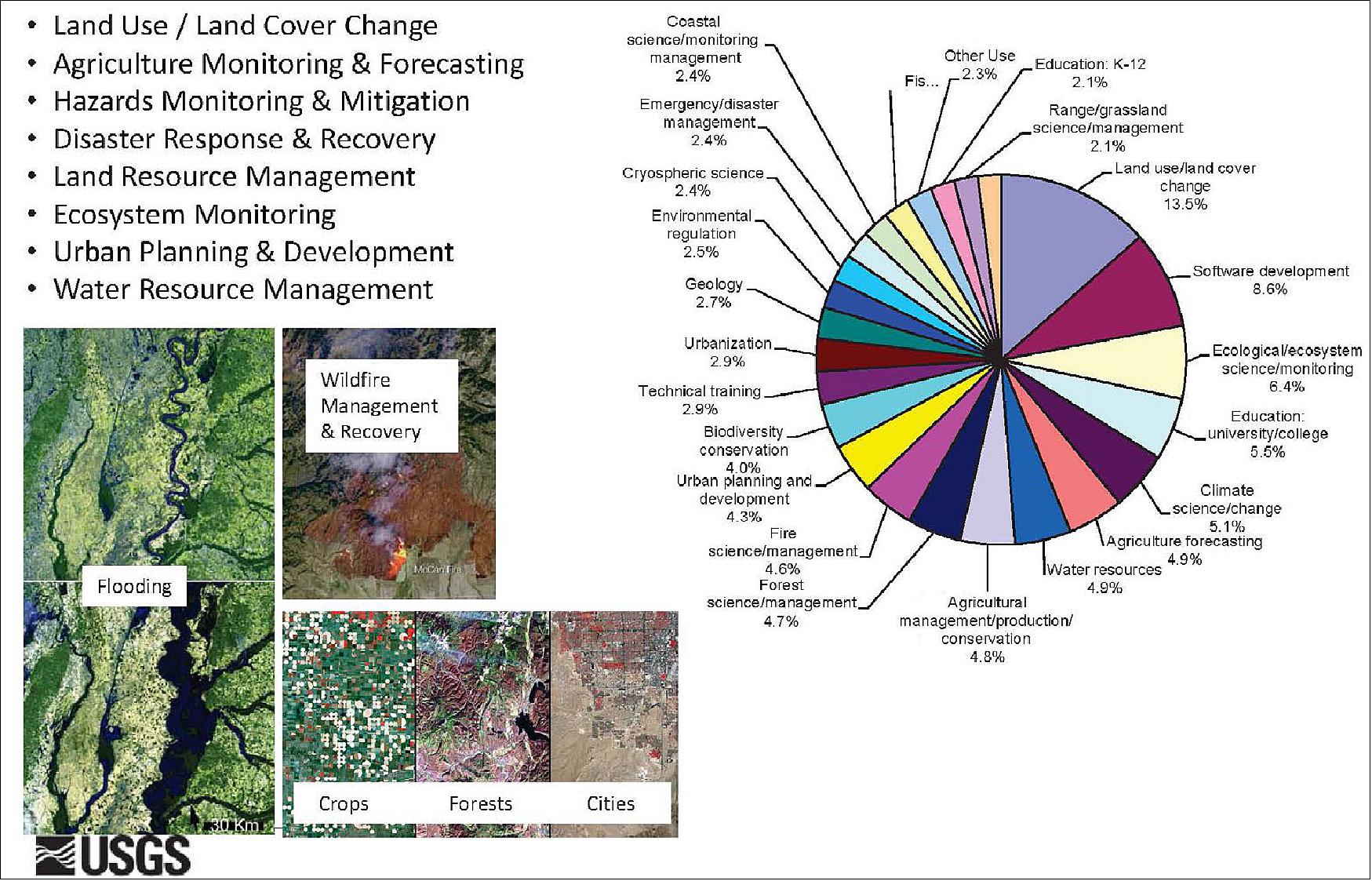
Coupled with dramatically lower costs for computing power, this move led to a revolution in use: Data analyses went from relatively small subscene/local studies, to regional, continental, and even global-scale studies. An analysis of how the various data are used is shown in Figure 18.
Integration with Data from Other Missions
Landsat 7 and NASA's Earth Observing System (EOS) flagship platform, Terra, also launched in 1999, were placed into orbit such that Landsat 7 is about 30 minutes ahead of Terra in the so-called “Morning Constellation”. This enabled the two satellites to capture congruent and near-synchronous data when vegetation and atmospheric conditions were similar.
This cross-mission integration is still producing benefits today, with a multitude of data fusion products from Landsat and the Moderate Resolution Imaging Spectroradiometer (MODIS) on Terra. One such outcome is the highly regarded Spatial and Temporal Adaptive Reflectance Fusion Model (STARFM), which has improved global agricultural monitoring. STARFM was designed to combine MODIS data with Landsat data to produce synthetic Landsat-like imagery on a daily basis.
Benefits from Landsat 7
Benefits from Landsat 7 fall into four main categories: technical, scientific, programmatic, and organizational. While some of the benefits were discussed earlier, the information that follows revisits these items and provides new introductions so that the full impact of Landsat 7 on Earth remote sensing across a wide range of categories may be easily grasped.
Technical Benefits: Lessons learned with the TM on Landsats 4 and 5 led to making the ETM+ the best-calibrated Landsat imager, allowing it to act as a cross-calibration source for other sensors on other platforms. Also, the implementation of the SSR onboard made possible the development of an automated LTAP that could yield nearly global, seasonal observations. This set the standard for all future Landsat missions. In the process, the Landsat 7 team developed and implemented a routine, randomly sampled image-assessment system to ensure data quality standards were being met.
Scientific Benefits: As discussed previously, the purposeful placement of Landsat 7 and the EOS Terra platform in the Morning Constellation, spaced about 30 minutes apart, allowed the respective Science Teams to optimize the scientific utility, e.g., capturing terrestrial ecosystems at multiple spatial and spectral resolutions under nearly identical plant physiological conditions.
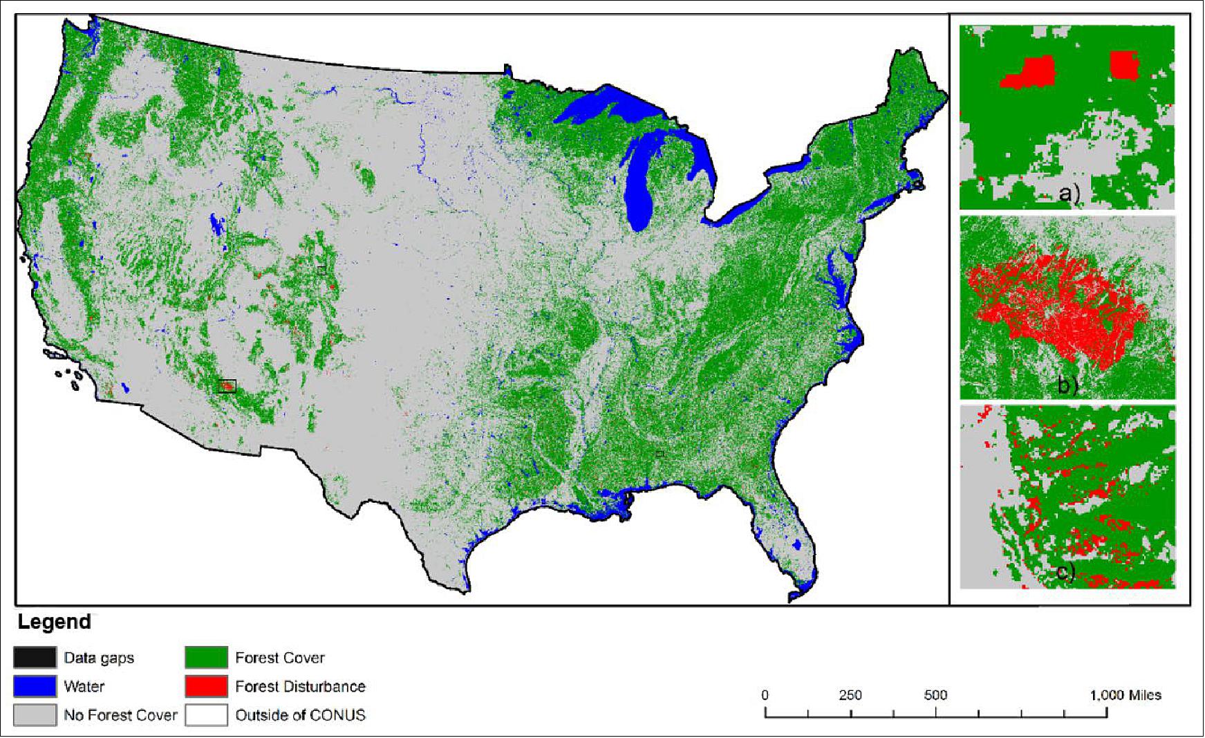
The major research area of plant response to stress came under the auspices of the North American Carbon Program, under which the North American Forest Dynamics (NAFD) Project generated integrated forest disturbance maps for the conterminous U.S. from 1986–2010, as represented in Figure 19. These time-integrated maps clearly demonstrated that some 20% of mapped locations experienced some form of disturbance over the study period, with consequences for the North American carbon cycle. 26)
In a significant development and with considerable planning and implementation to acquire as much imagery of the continent as possible, over 1000 Landsat 7 scenes were chosen to create the then-highest resolution image mosaic of Antarctica, the Landsat Image Mosaic of Antarctica (LIMA). LIMA was instituted as part of the International Polar Year (2007–2008). Supporting organizations included NASA, USGS, and the British Antarctic Survey. The program had several goals, including supporting polar research and an outreach component designed to make Antarctica and physical changes there more accessible to the general public. Images obtained for LIMA include a vast array of high-resolution images suitable for such purposes, as exemplified in Figure 20. As Robert Bindschadler [NASA’s Goddard Space Flight Center—LIMA Project Lead] said at the time, “The revolutionary concept of systematic collection of Landsat 7 data timed to optimize anticipated scientific applications will make possible a global monitoring of the cryosphere with a dataset heretofore only available in limited regions.”
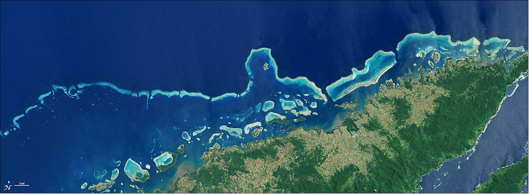
Another first was the Millennium Coral Reef Mapping Project in 2006, in which Landsat 7 data were used to create a first-of-its-kind global survey of coral reefs. The research lead on this project, Frank Muller–Karger [University of South Florida, Director of the Institute for Marine Remote Sensing] commented in 2015 that, “Until we made the map of coral reefs with Landsat 7, global maps of reefs had not improved a lot since the amazing maps that Darwin drafted.” An example of an image that facilitated this research is shown in Figure 21. As with LIMA, considerable effort went into scheduling and sensor preparation to allow a wide array of scenes.
In general terms, Landsat 7 thermal infrared imagery with its 60 m resolution could be used to estimate evapotranspiration (i.e., water uptake and release) from crops and the soil they grow in—down to the level of individual agricultural fields. This enabled major advances in water use management (i.e., irrigation practices).
Further, the 30-m resolution of the ETM+ provides an excellent match with the scale of human activities, so the massive increase in holdings in the Landsat image archive allows a clearer look at the impacts of those activities on the planet’s various systems. Being able to translate from local, to regional, continental, and even global scales depending on the phenomena being investigated was a welcome development.
Programmatic Benefits: With the advent of Landsat 7, contributions to global change research were considered of major importance by providing detailed human-scale measurements of land conditions and dynamics. The return to government operations and contemporary mission configuration facilitated this major transition to Landsat scientific research, not least because of the massive changes in data access policies and their subsequent implementation.
When Landsat was first proposed it was mainly considered an applications—not science—mission. There was a first call for proposals in 1971 that lasted until 1972 and explored many uses. In 1973 Congress directed NASA to use Landsat for agricultural monitoring, after the then-Union of Soviet Socialist Republics (USSR) caused difficulty in the commodities (e.g., wheat) market.
Although it was clear that land dynamics probably played important roles in Earth system science, Landsat was rarely used for this purpose until the late 1980s. Indeed, the agricultural focus lasted until Landsat was commercialized in 1986, but when Landsat was returned to government operations in 1992, NASA directed it to service the needs of Earth system science.
Organizational Benefits: For the first time in the Landsat program, NASA and USGS selected a Science Team to support the Landsat 7 mission. This science team represented myriad scientific interests including agriculture, cryosphere, clouds, coastal zones and coral reefs, tropical and temperate forestry, land cover, geography, and geology, as well as foundational support for radiometric calibration of optical and thermal measurements and atmospheric corrections. The Science Team is now in its third complement, and continues to support the mission admirably.
The work of these team members, as well as NASA and USGS staff, led to the development of Landsat data products suitable for time series studies at regional-to-global scales, clearly demonstrating the benefits of interorganizational communication and participation.
The Future of Landsat 7
As with all such missions, end-of-life planning is a major part of the mission. Throughout its lifetime, Landsat 7 has undergone several orbital maneuvers to ensure that the local-mean-time (LMT) data acquisitions are maintained. The final such “Delta-I” (i.e., change in inclination) maneuver took place on February 7, 2017. From that point forward, the satellite’s orbit has begun to slowly degrade (lower) such that by 2020 the LMT will fall back from the desired 10:00 AM LMT to about 9:15 AM.
By the time of the planned launch of Landsat 9 late in 2020, Landsat 7’s orbit will have degraded such that Landsat 9 can move into the 705-km ) “standard” orbit altitude, and take Landsat 7’s place in an orbit that allows data to be collected eight days out of phase with Landsat 8 (with two satellites in orbit, a Landsat scene is collected over every location on Earth every eight days). Landsat 7’s 9:15 AM LMT acquisition will preclude acquiring high-quality and heritage-continuing data, and the satellite will be decommissioned. (To minimize orbital debris, space policy requires that adequate propellant be reserved to conduct orbit adjustment burns to rapidly remove a satellite from orbit once it is declared inoperable.)
In a new era of efficiency and competition for limited resources, plans are underway to explore the possibility of using NASA's Restore-L Robotic Servicing Mission 27) to refuel and service Landsat 7, primarily to ensure successful decommissioning, but also to provide the possibility of turning the satellite into a transfer radiometer. This would allow it to act as a calibration instrument for Landsats 8 and 9, and perhaps even extend its scientific utility.
Earth Insights
With capabilities such as those afforded by the Landsat program worldwide,Earth system changes are observed in both real-time and across time, the latter providing a longer-term view on how Earth’s various systems interact with each other across long (by human standards) time scales. Many systems are affected, including “....human health, agriculture, climate, energy, fire, natural disasters, urban growth, water management, ecosystems and biodiversity, and forest management,” according to NASA. 28)
In summary, among its other significant advances, we note that:
- by continuing the increasingly long record of land-surface phenomena, Landsat 7 offered mission continuity for the Landsat program;
- with the absolute calibration provided by its onboard capabilities, Landsat 7 provides not only high-quality data but also on-orbit, cross-calibration capability for other Earth-science missions;
- with its repeated data acquisitions under sunlit, cloud-free conditions, Landsat 7’s global survey mission offered a closer look at our planet’s interacting systems; and
- by providing free access to already acquired scenes, interested parties—be they researchers or decision makers—have enhanced ability to manage Earth’s resources and, potentially, to reduce the impact of human activities on vital systems.
From its inception to the present day the Landsat program has provided us with broad and deep insights into our planet’s land surfaces and their uses. Each successive Landsat platform has made contributions to relevant and useful data sets. Landsat 7 continued that trend, and its follow-on missions further build upon that legacy: Landsat 8 is currently in orbit and Landsat 9 is scheduled for launch in late 2020.
Absent the sheer volume and high quality of such moderate-resolution data, we would not possess our current deep and broad understanding of our home planet’s landsurface systems and how they interact with other Earth systems (Ref. 24).
• July 2, 2019: Thanks to the Moon, the Sun, and gravity, the place where the land meets the sea is not a fixed line. What we see on a map is just a representation of where mean sea level is found, and the coast of any landmass is really a moving target between low and high tides. This ever-shifting region is known to scientists as the intertidal zone. 29)
- The world’s intertidal zones include an array of ecosystems: sandy beaches, rocky shores, tidal pools, mudflats, seagrass beds, mangrove forests, and fringing coral reefs. So many life forms have adapted to this transitional place, and they play a critical role in the food chain and in nutrient and carbon cycling. For instance, the intertidal zone is an indispensable feeding ground for shorebirds, particularly during migration.
- For humans, the zone provides recreational spaces and the first line of defense against the sea. Knowing the width and height of the intertidal zone aids in tsunami preparedness, storm surge risk management, current modeling, and ecological habitat mapping. Yet this region has largely been missed in most mapping efforts, falling between well-mapped dry land and bathymetry (depth) measurements of the ocean.
- Led by Robbi Bishop-Taylor and Stephen Sagar, the team created the first automated, open-source method for deriving intertidal zone elevations. Then they made the first nationwide coastal elevation model for Australia, the National Intertidal Digital Elevation Model (NIDEM), covering more than 15,000 km2 (5,800 square miles) of coast. The work was published in the journal Estuarine, Coast and Shelf Science.
- “The rise and fall of tides can be used to trace the 3D shape of the intertidal zone,” Bishop-Taylor explained. “By sorting 30 years of Landsat satellite images using a tidal model, we can reveal exactly what areas of the coastline are exposed at different levels of the tide.”
- Building on earlier work that used Landsat to map the horizontal extent—the x and y directions—of the intertidal zone, the Geoscience Australia team applied knowledge of the tidal range and of the presence or absence of seawater during the tidal cycle to model the elevation—the “z”—relative to mean sea level. The accuracy of this approach for tidal flats and sandy shores is high, approaching that of lidar-derived elevations. For rocky shores and places where the tidal model does not capture the complex or extreme tidal patterns, NIDEM is a bit less accurate.
- From coastal risk mitigation to ecological conservation, NIDEM stands ready to help coastal managers. For instance, researchers at James Cook University have already incorporated the full NIDEM data set into the elevation model for the Great Barrier Reef and Queensland coast. The Queensland Government used an earlier version of this elevation model for regional habitat mapping. And Sagar noted that his team has introduced NIDEM to the hydrographic surveying community as a cost-effective means to fill the gap between ship-based bathymetry measurements and terrestrial elevation data.
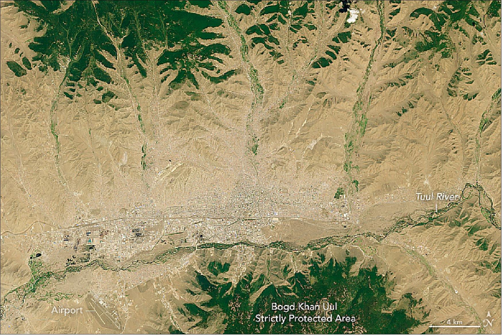
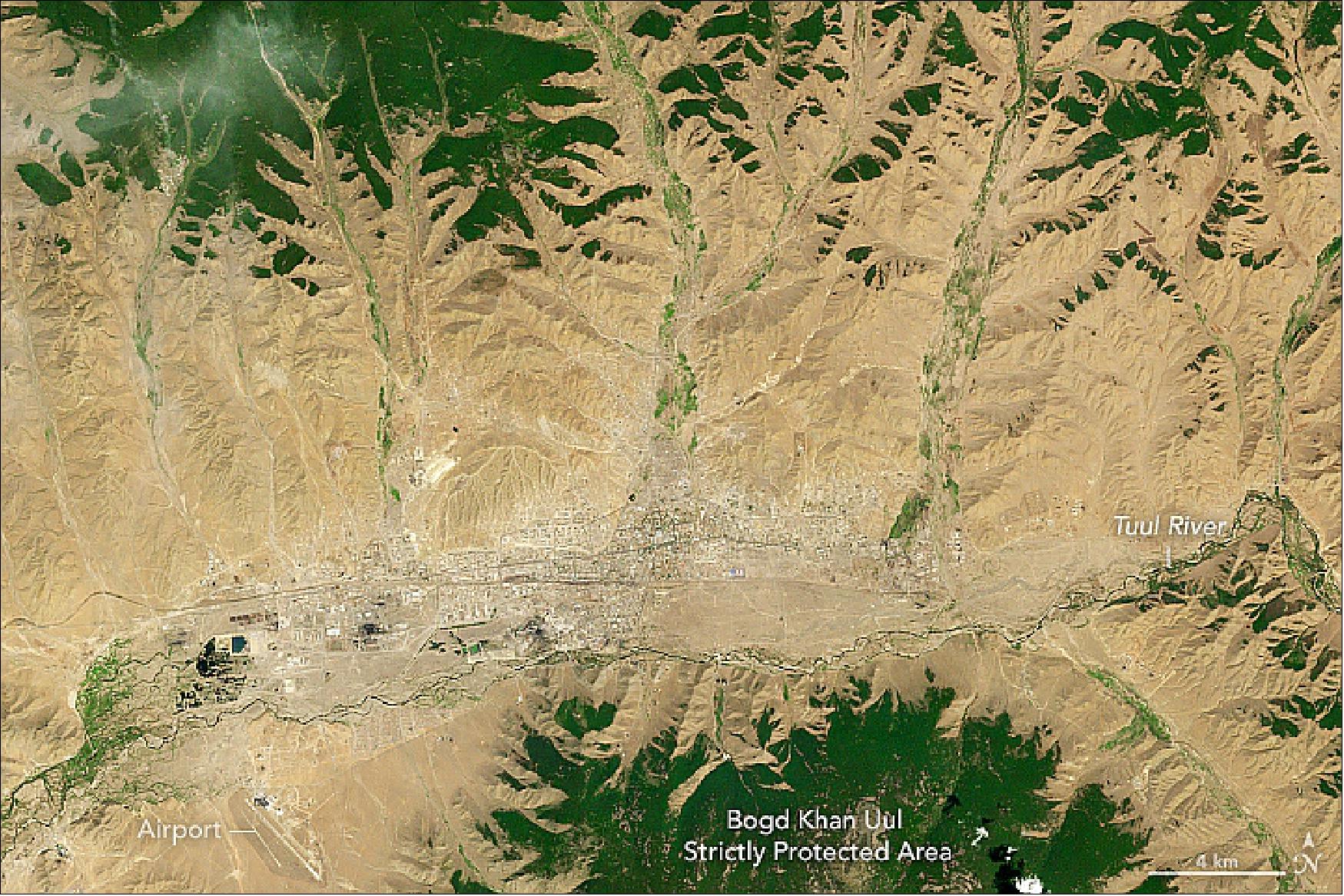
• June 4, 2019: Mongolia’s capital, Ulaanbaatar, sits near the confluence of the Selbe and Tuul rivers on a plateau at the foot of a large, forested mountain. This was not always the case. When the town was initially established in the 1600s, it was a migratory settlement built as a center for Buddhist priests. It changed locations more than two dozen times. 30)
- Ulaanbaatar settled into a permanent location in the 1700s, but it remains a place of rapid change. These days, the growth is mostly outward into low-density neighborhoods that have emerged on the fringes of the city, particularly in river valleys and hillsides north of the city center. Migrants typically set up gers, the circular, herder tents that nomadic people have traditionally used in the Mongolian steppe. In contrast, the core of the city features Soviet style architecture—grand neoclassical government buildings and grids of rectangular, multi-story apartments that were mostly built in the 1960s.
- Several teams of scientists have used Landsat images to monitor how the city—particularly the ger districts—have changed over several decades. According to some estimates, ger districts now hold more than 60 percent of Ulaanbaatar’s population.
- The Landsat-8 and -7 satellites captured these natural-color images of the city in 2018 and 2000, respectively. Notice the development in the river valleys (green linear features) that lead out of the city. Note also how forested areas in the hills north and south of the city have lost tree cover over the years, probably due to people harvesting wood to heat their homes.
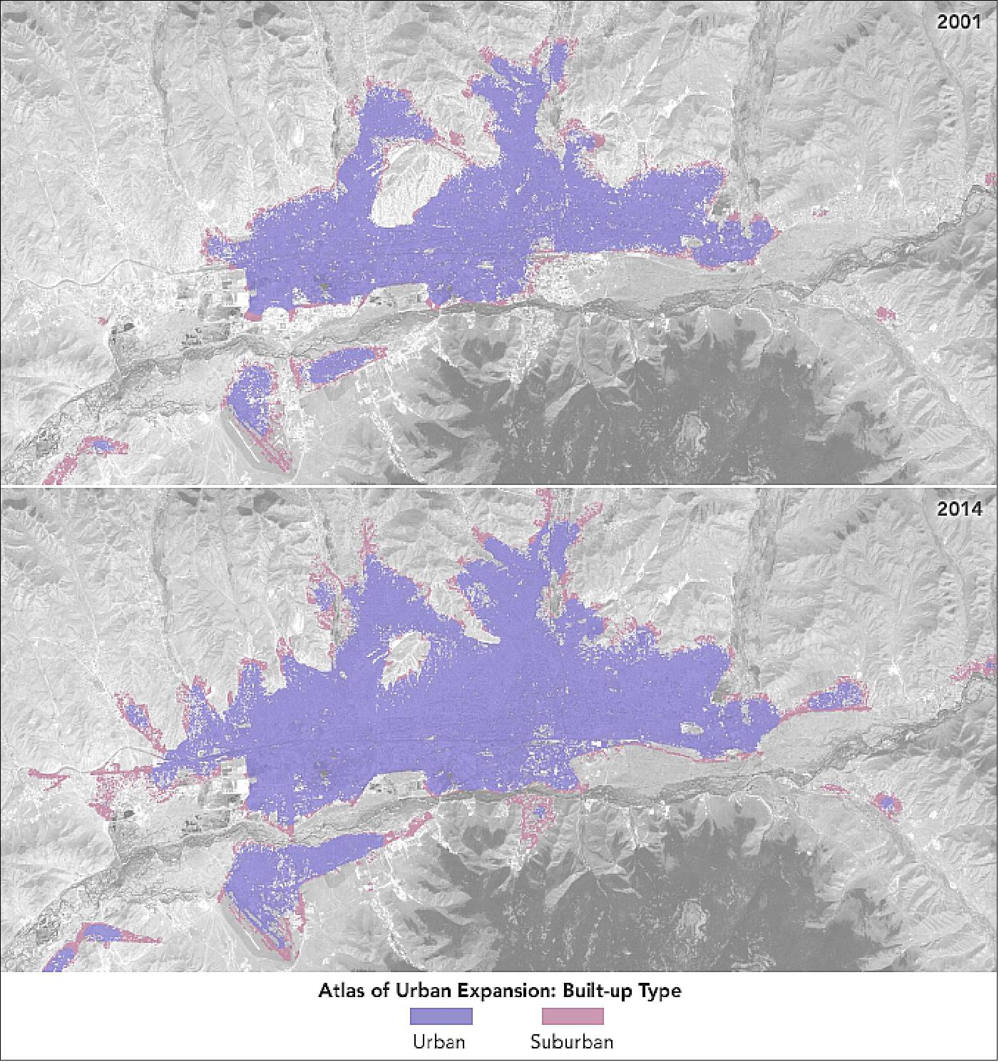
- Migrants from the countryside have been moving into the city in large numbers since 1992, the year that Mongolia adopted a free-market system and abandoned central government control of the economy. Around that time, lawmakers passed a bill that entitled every Mongolian citizen to 0.7 hectare of land within a city for free, a law that helped entice hundreds of thousands of people to move. Meanwhile, cold spells known as dzuds caused such severe damage to livestock across multiple winters that many rural Mongolians were forced to move to survive.
- The rapid migration of people into the city has come with consequences. Many of the gers that people have set up are heated with wood or coal, which has significantly increased air pollution. Ulaanbaatar’s air is among the most polluted in the world, and particulate concentrations in the winter air have occasionally exceeded safe levels by more than 100 times. In addition, many homes in ger districts lack access to electricity, paved roads, and sewers.
• February 21, 2019: KBR, Inc. (formerly Kellogg Brown & Root) of Houston, TX, announced today that its global government services business, KBRwyle, has been awarded a $19 million contract by the U.S. Geological Survey (USGS) to support flight operations for its Landsat-7 satellite. 31)
- The Landsat-7 satellite is part of the Landsat program, a joint initiative of the USGS and NASA. Landsat satellites provide space-based images of the Earth's land surface, collecting valuable data that helps reduce hunger on Earth, enhances how quickly emergency response teams stabilize fires, and aids scientists in understanding humanity's impact on the planet.
- Under this contract KBRwyle will perform flight operations, system maintenance, testing, and sustainment engineering activities to support the on-orbit Landsat 7 spacecraft and payload. KBRwyle will also operate and maintain the Mission Operations Center (MOC) ground systems and backup Mission Operations Center (bMOC). Additionally, the company will continue to participate in a NASA/USGS initiative to robotically refuel the Landsat 7 spacecraft.
- KBRwyle will primarily perform this work at NASA's Goddard Space Flight Center in Greenbelt, Maryland, as well as at its office in Columbia, Maryland. The firm-fixed-price, time and materials contract's period of performance is one base year with four option years. The maximum value of this contract is $19M if all options are exercised.
- "KBRwyle is proud to continue supporting this program that equips society with critical data about the Earth," said Byron Bright, KBR President Government Services U.S. "Landsat satellites tell the story of our planet. They capture data from current events and show the evolution of our environment, providing invaluable information to decision makers."
- Landsat satellites have acquired data from across the globe for more than four decades. The National Satellite Land Remote Sensing Data Archive (NSLRSDA) at the USGS Earth Resources Observation and Science (EROS) Center holds the single most geographically and temporally rich collection of Landsat data in the world, currently holding more than six million Landsat scenes.
- KBRwyle provides technical support services to the USGS EROS Center. At this center, KBRwyle maintains and operates the Landsat-7 and -8 ground processing system while helping to develop the next generation Landsat-9 ground system in support of a planned 2020 launch. The EROS Center processes and distributes data from the Landsat archive and other Earth observing satellites, as well as other forms of geographic science products and information.
- KBRwyle has partnered with NASA and USGS for more than two decades to help Landsat satellites provide imagery—a unique resource for those who work in agriculture, geology, forestry, regional planning, education, mapping, and global change research. KBRwyle began its legacy of support with Landsat-5 in 1994, operating the satellite to set a new Guinness World Record for the longest-operating Earth observation satellite.
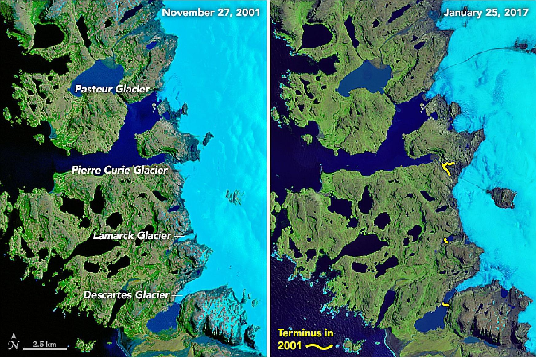
• April 27, 2018: The Kerguelen Islands rise from the southern Indian Ocean, not far from the “Furious Fifties.” As a result, the Kerguelens are often shrouded by clouds, making it hard for satellites to get a good look at the shrinking ice cap on the archipelago’s main island, Grand Terre. 33)
- “There are limited in situ observations here, so without satellite images we do not have much to go on,” said Mauri Pelto, a glaciologist at Nichols College who has been analyzing satellite imagery of glaciers since the 1980s. “Radar can see the size of glaciers to some extent, and we can measure height, but without good imagery, we can’t measure velocity.”
- Over 16 years, each of the main glaciers in the images retreated. Near the top, the 600-meter-retreat of Pasteur Glacier means that its ice front now terminates on land, not in the water. To the south, Pierre Curie Glacier retreated about twice as far. Lamarack Glacier retreated by 1100 meters, its terminus also trading water for land, while Descartes Glacier retreated by 1000 meters through a narrow arm of a lake. Notice the appearance of nunataks—peaks of rock that now protrude from the ice surface.
- A study published in 2015 confirmed that the retreat of this ice cap is due primarily to changes in snowfall. Since the 1970s, precipitation on the Kerguelen Islands has not been sufficient to offset the melting of snow and ice. Similar losses are occurring to glaciers in other southern subpolar regions, such as in New Zealand and Patagonia.
• As of 15 April 2018, Landsat-7 is 19 years on orbit.
• March 22, 2018: In a part of the Amazon rainforest that reaches into northeastern Peru, there are no roads cutting through the vegetation and no visible patches of deforestation. “When you see it from the air, it appears to stretch to the horizon,” said Corine Vriesendorp, a conservation ecologist at the Field Museum. 34)
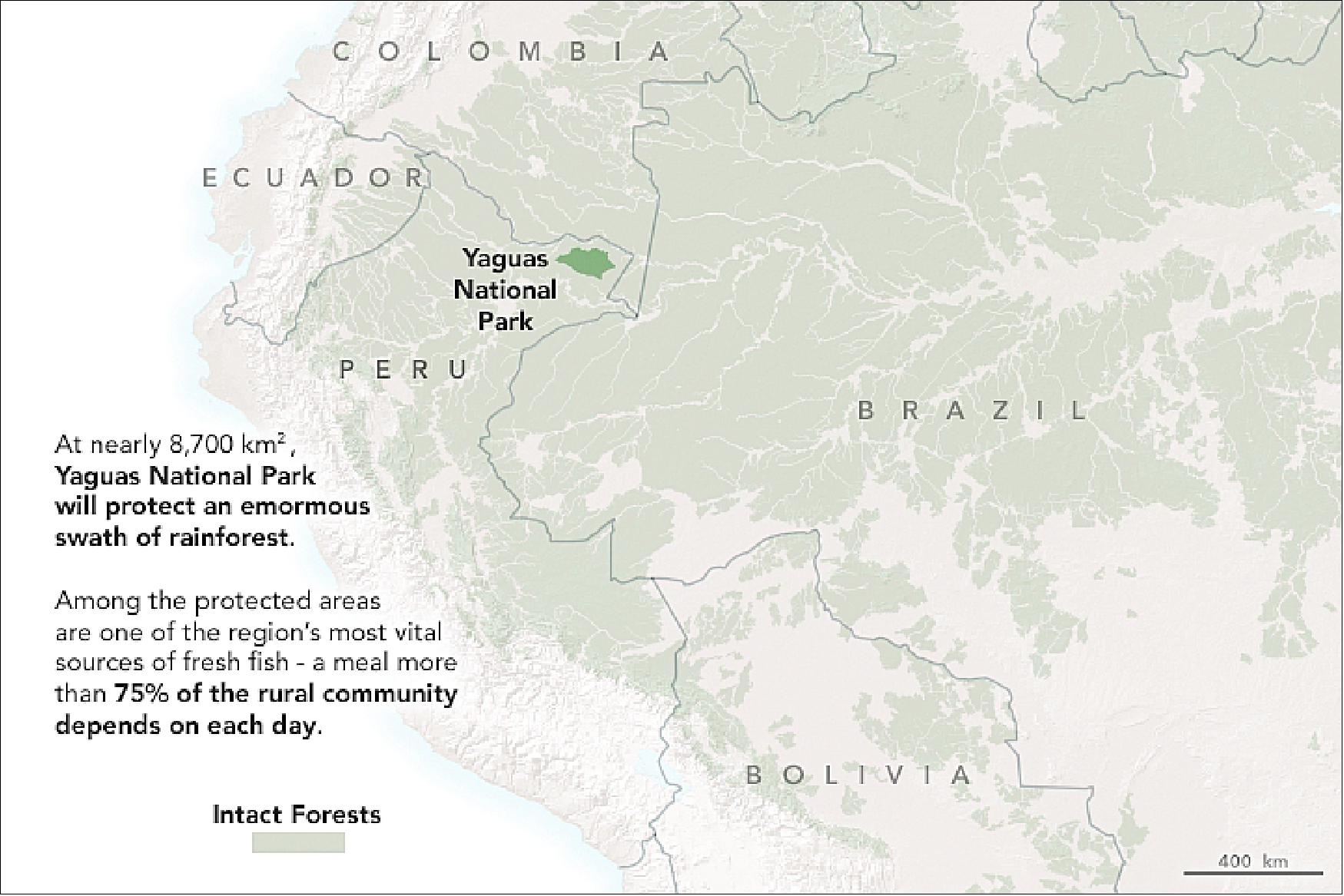
- Formally established in January 2018, Yaguas National Park helped ensure that more than 2 million acres (809,370 ha) of Peruvian Amazon forest stay intact. The park’s boundaries are shown here, atop a map of aboveground forest biomass. Satellite data and models were used to estimate the density of woody material (Figure 29); dark green areas are denser than light green areas. The map of Figure 30 puts the park amidst the wider forested areas.
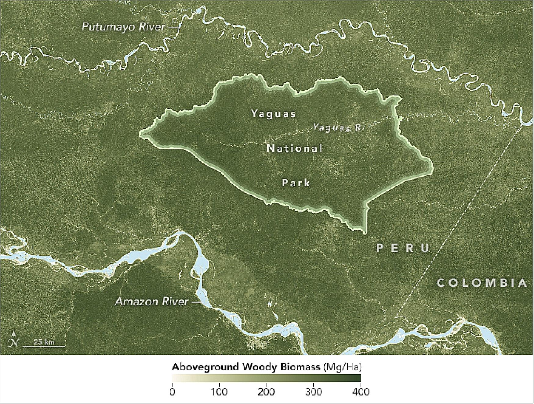
- These intact forests are important for supporting biodiversity. They give plants and animals adequate space to maintain healthy populations and to continue to evolve as they have over millions of years. Uninterrupted or “connected” forests can even help species respond to climate change by allowing them to migrate to areas with more moisture or higher, cooler elevations.
- The park does not just protect flora and fauna; it preserves an entire watershed, which Vriesendorp called “an increasingly rare conservation opportunity.” The watershed extends the entire 200 km from the headwaters to the mouth to the Yaguas River. “That’s about the same distance as driving from Chicago, Illinois, to Madison, Wisconsin, or from New York City to Atlantic City, New Jersey,” Vriesendorp said.
- Part of the Yaguas River is visible in this image, acquired on August 16, 2017, by the Operational Land Imager (OLI) on the Landsat-8 satellite. A few oxbow lakes (dark brown) are visible near the river (light brown). These bows form when the river begins to flow along an "easier" route and cuts off one of its meanders.
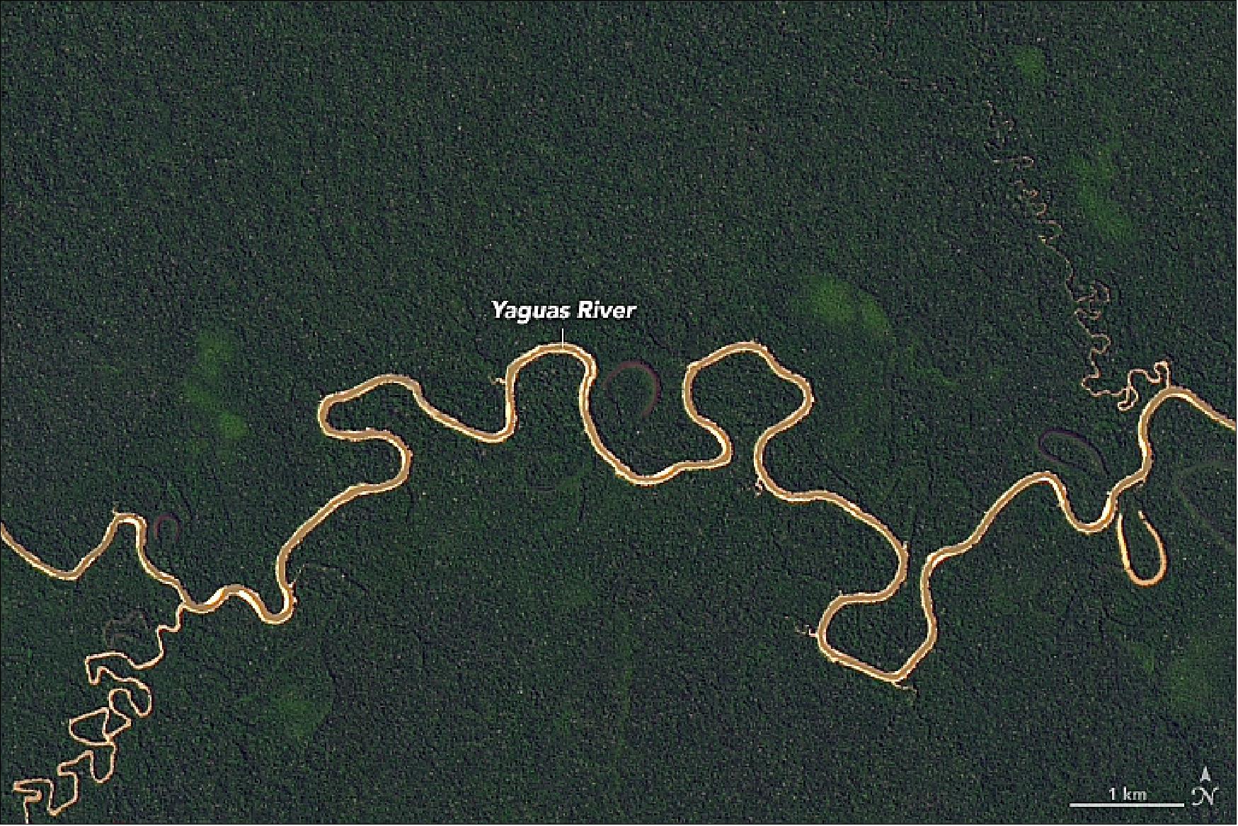
- Abandoned meanders are likely also the reason for the light green patches that appear “bare” on either side of the Yaguas River. These are peatlands—a soil-like mixture of partly decayed plant material that can build up in the abandoned river meanders. If it becomes dried or burned, it can be a significant source of greenhouse gases such as carbon dioxide. Peatlands are extensive along the Yaguas River, and also along the larger Putumayo River to the north.
- “Ten years ago, we were just beginning to realize that there were important peat deposits in the Peruvian Amazon,” Vriesendorp said. “Although there has been no comprehensive mapping of the Putumayo’s peatlands to date, it is likely that the below-ground carbon stock is immense.”
- Note: March 21 is the International Day of Forests, a day established by resolution of the United Nations General Assembly to celebrate and raise awareness of the importance of all types of forests.
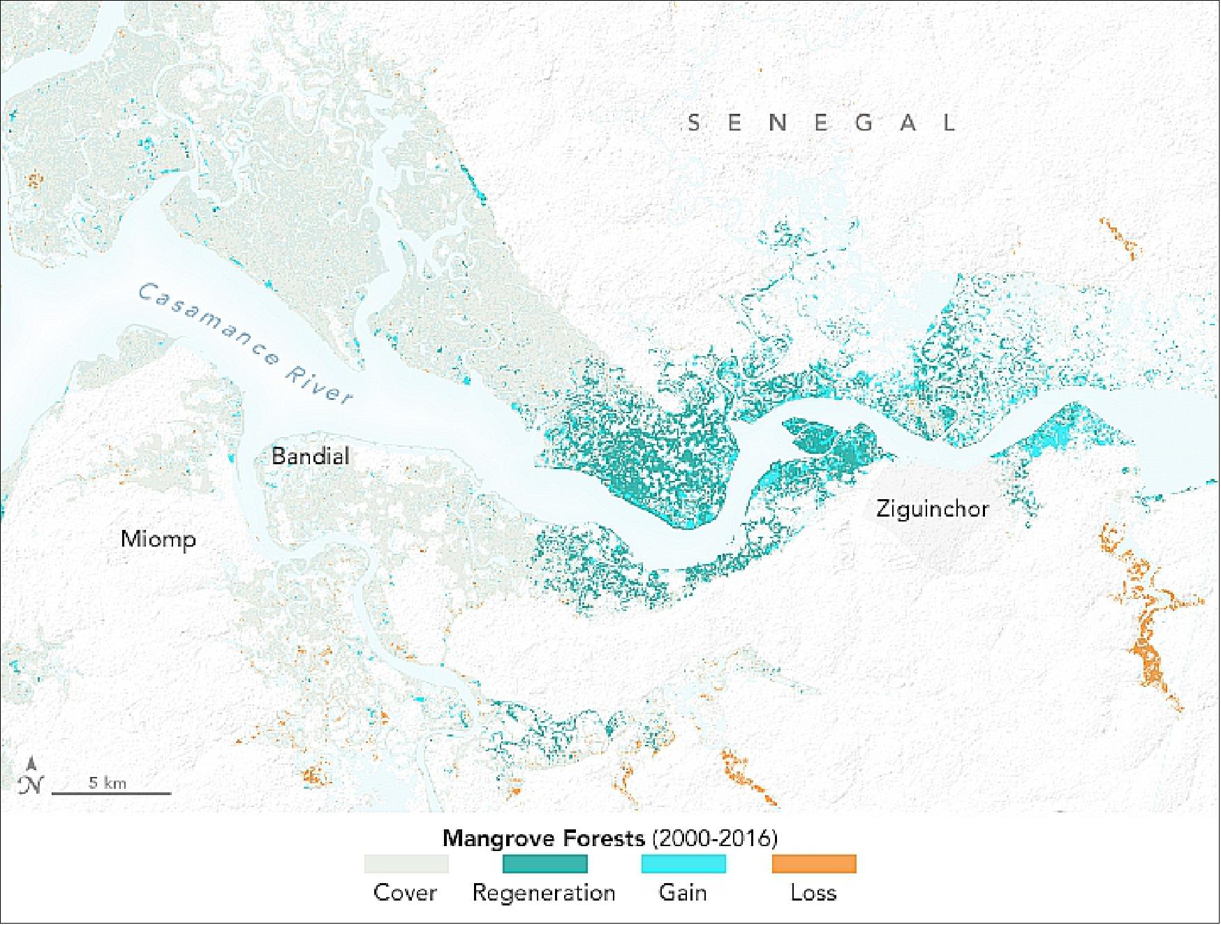
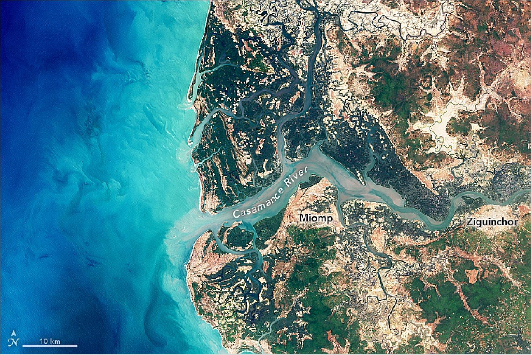
• March 21, 2018: Many of Senegal’s largest rivers are flanked by corridors of green and interlaced with networks of sinuous creeks and streams. These lush green areas are havens for mangroves—short, shrubby trees with waxy leaves and tangles of finger-like roots that rise from shallow tidal areas. 35)
- The blend of land, water, and wood that define Senegal’s mangrove forests are not just beautiful; they are important. Mangroves store large amounts of carbon. Studies have shown that mangrove forests sequester at least two to four times more carbon than other tropical forests. They also provide breeding grounds and nurseries for fish, prevent erosion during tropical cyclones, and help cleanse waters of pollutants.
- While scientists estimate that Earth lost at least 35 percent of global mangrove habitat between 1980 and 2000 (often due to aquaculture and other coastal development), there are signs that these ecosystems are surviving and even retaking lost ground in some areas. For instance, Senegal’s mangroves have experienced significant regeneration and expansion since 2000, according to a satellite-based analysis by NASA scientists Lola Fatoyinbo and David Lagomasino. Over the 16-year period, the scientists measured an expansion totaling 48 km2, or 2 percent. They observed regeneration across 148 km2, an increase of 6 percent.
- This regrowth after decades of loss likely had several causes, the scientists say. A prolonged and damaging drought in the 1970s and 1980s killed many of Senegal’s mangroves; the water became too salty when the freshwater flow from rivers dwindled. The easing of that drought allowed mangroves to recolonize many areas. Meanwhile, the normal deposition of sediment along river edges has created new shallow areas that mangroves have been able to colonize.
- Senegal has established parks and used other conservation measures to protect some mangroves from being damaged or cleared. Several non-governmental organizations and environmental groups also launched mangrove-planting projects. The Saloum and Casamance deltas, in particular, have been a focus of “blue carbon” restoration efforts, with one organization reporting that it planted more than 79 million trees in the two deltas.
- The map of Figure 32 shows how mangrove forests along the Cassamance River changed between 2000 and 2016. The analysis is based on Landsat satellite observations of the “greenness” of vegetation, or the NDVI (Normalized Difference Vegetation Index). Areas marked as gain (teal) had no mangroves in 2000 but measurable growth by 2016. Areas marked as having regenerated (green) had mangroves in 2000 that became significantly greener and denser by 2016. The natural-color image of Figure 33 was acquired by OLI (Operational Land Imager) on Landsat-8 on March 5, 2018.
- “For decades, there has been so much negative news about losing mangroves that it is easy to forget that these are plants that are almost perfectly designed to trap sediment and colonize empty mudflats,” said Fatoyinbo. “The regeneration of mangrove ecosystems is something we are actually seeing in several parts of the world now.”
• September 14, 2017: Engineers have successfully completed recovery efforts of the Landsat-7 SSR (Solid State Recorder) anomaly that occurred on September 13, 2017. The satellite resumed nominal imaging operation as of September 13 (DOY256) at 22:09 UTC (5:09 pm CST) and data are available to download from EarthExplorer, GloVis, or the LandsatLook Viewer. 36)
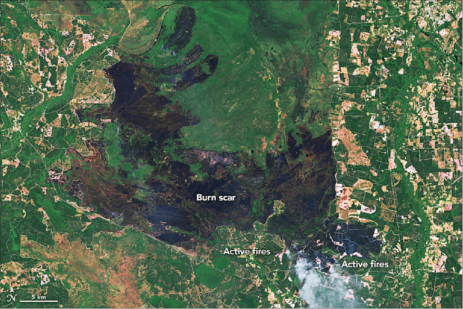
• May 11, 2017: More than a month after being ignited by lightning, the West Mims fire continues to burn along the Florida-Georgia border. On May 8, 2017, the ETM+ (Enhanced Thematic Mapper Plus) on the Landsat 7 satellite captured this image of the wildfire, most of which has burned within the Okefenokee National Wildlife Refuge. The Okefenokee National Wildlife Refuge has a size 1,627 km2 located in Charlton, Ware, and Clinch Counties of Georgia, and Baker County in Florida, United States. 37)
- According to InciWeb, the burned area grew from 100,500 acres (401 km2) on May 2 to more than 133,700 acres (541km2) on May 8. A closer view of the burn scar is visible in the first photograph below, acquired from aircraft on April 25, 2017.
- The lightning-caused fire was reported on April 6, 2017, approximately 4 km northeast of the Eddy Fire Tower in the Okefenokee National Wildlife Refuge. The Southern Area Type 1 Red Incident Management Team is managing the fire with Georgia Forestry Commission, Greater Okefenokee Association of Landowners (GOAL), U.S. Fish and Wildlife Service, Florida Forest Service, and U.S. Forest Service.
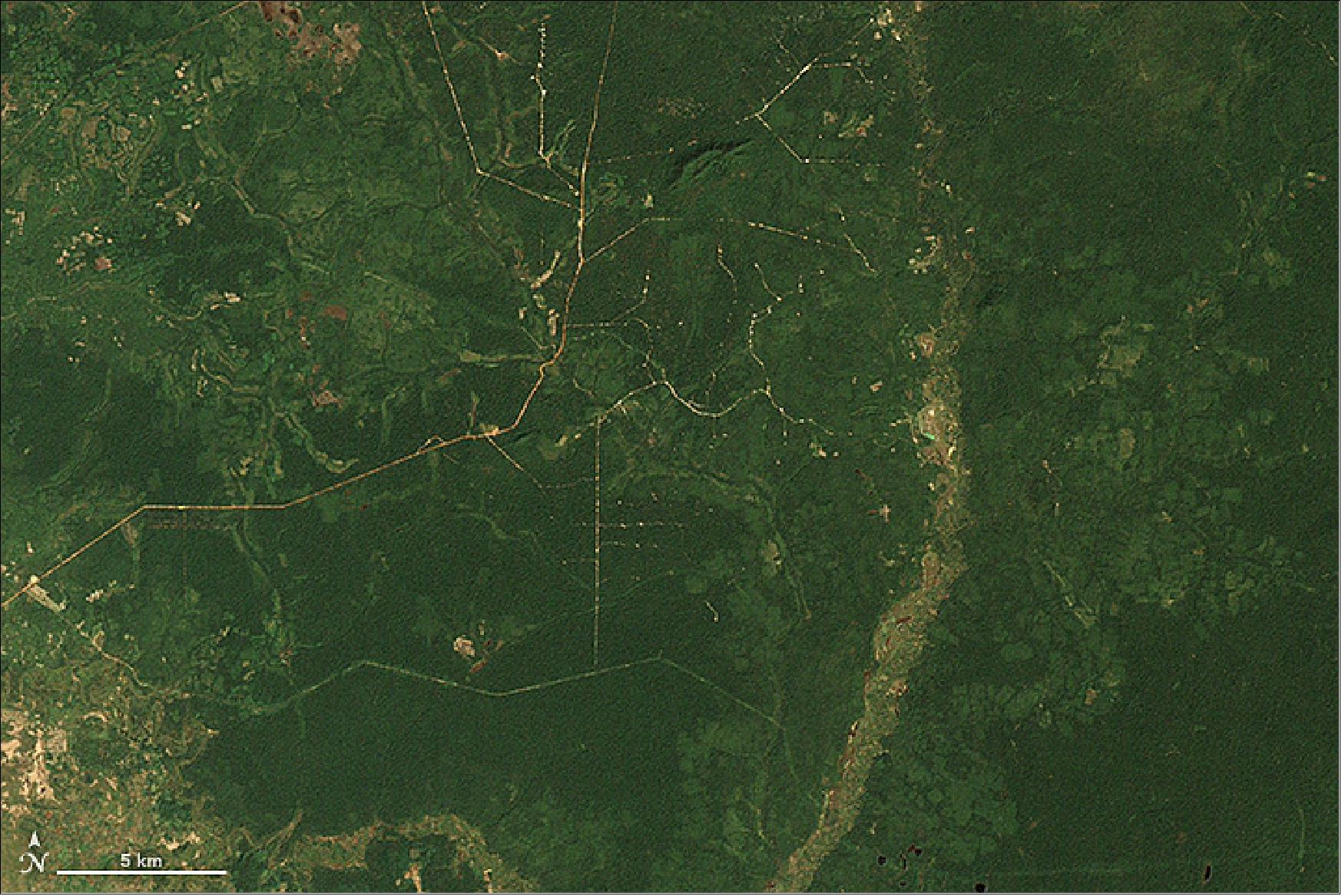
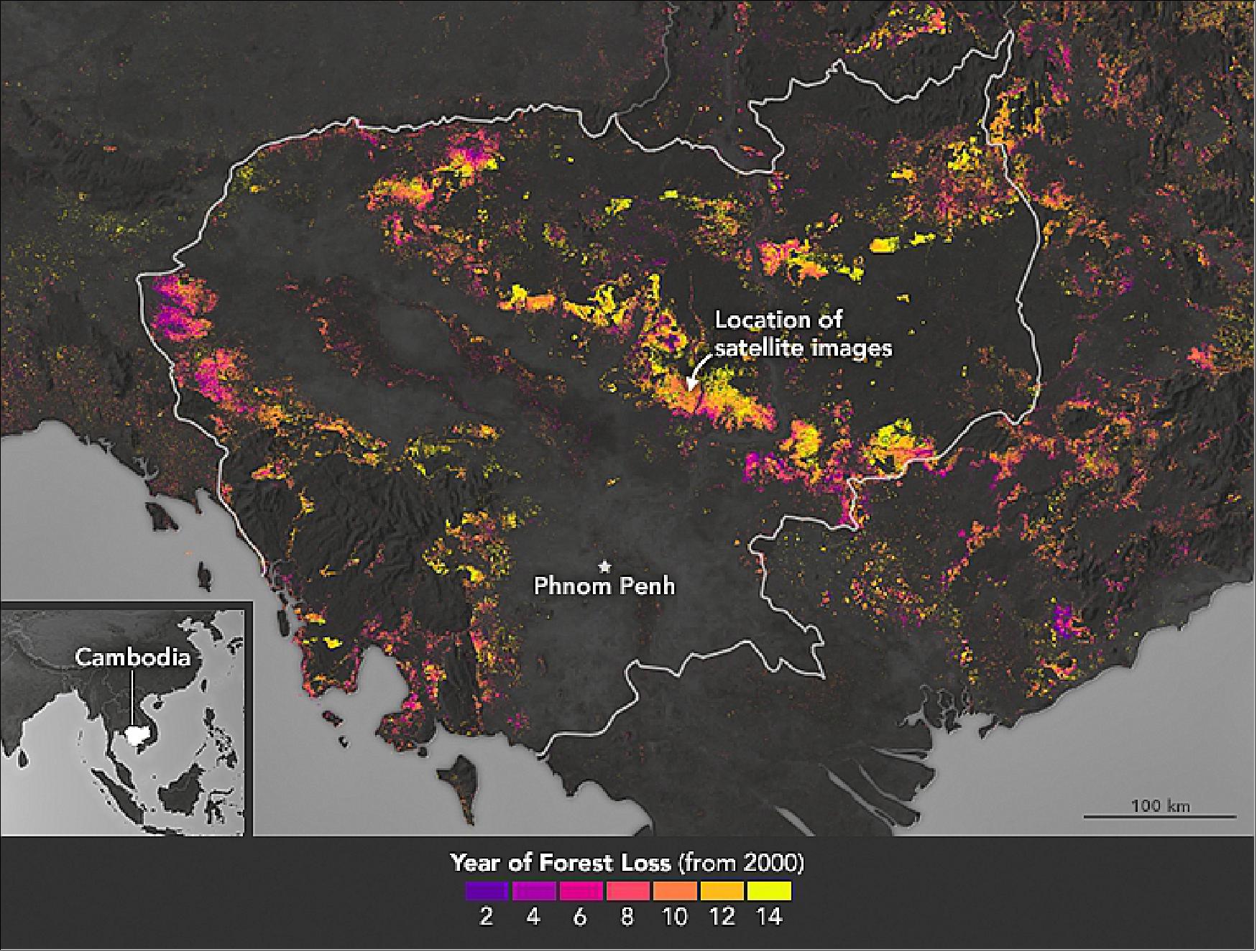
• January 10, 2017: Cambodia has one of the fastest rates of forest loss in the world. In broad swaths of the country, densely forested landscapes—even those in protected areas—have been clear-cut over the past decade. Much of the forest has been cleared for rubber plantations and timber. 38)
- Scientists from the University of Maryland and the World Resources Institute’s Global Forest Watch have been using Landsat satellite data to track the rate of forest loss on a global scale. Though other countries have lost more acres in recent years, Cambodia stands out for how rapidly its forests are being cleared.
- Between 2001 and 2014, the annual forest loss rate in Cambodia increased by 14.4 %. Put another way, the country lost a total of 1.44 million hectares—or 14, 400 km2—of forest. Other countries with accelerating rates of forest loss include Sierra Leone (12.6 %), Madagascar (8.3%), Uruguay (8.1%), and Paraguay (7.7%).
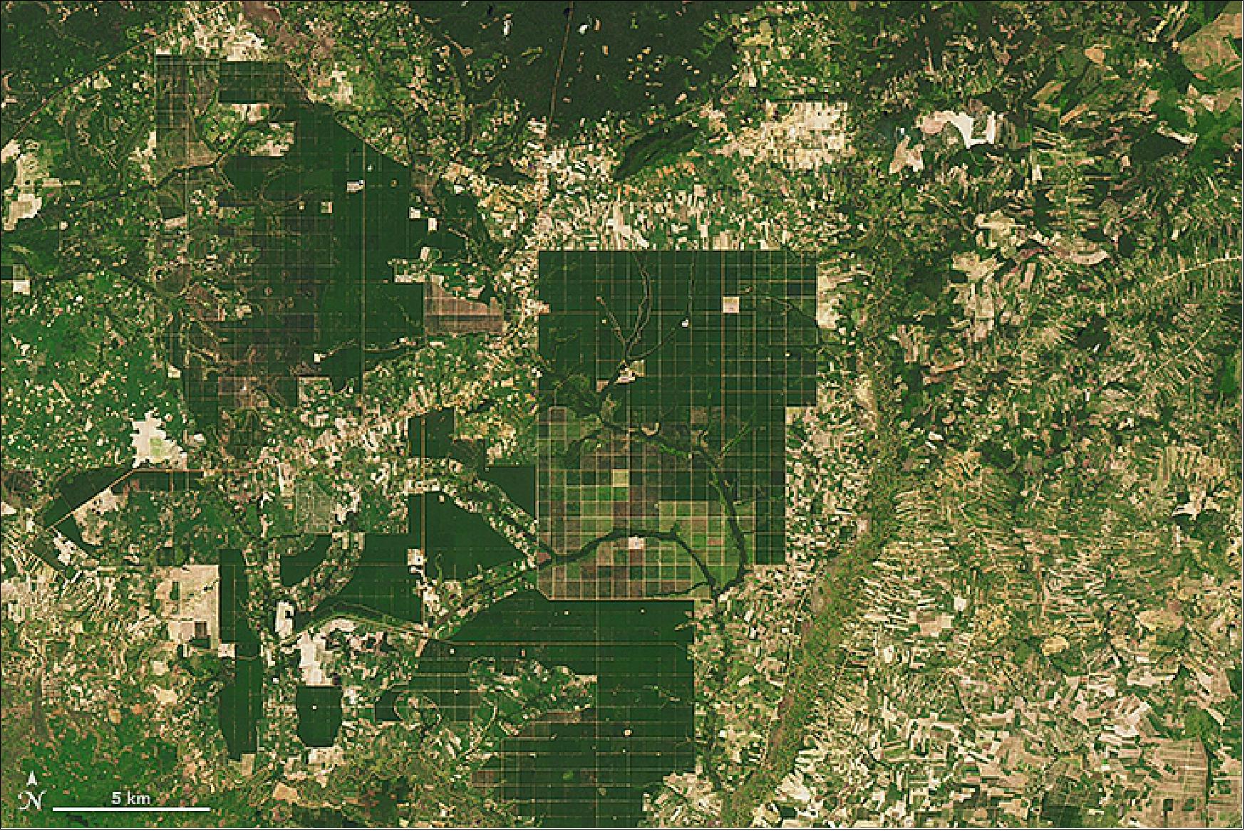
- The transformation of Cambodia’s landscape has been profound, as revealed by this pair of Landsat images. The image of Figure 35, captured by Landsat 7’s ETM+ (Enhanced Thematic Mapper Plus) on December 31, 2000, shows intact forest near the border of the Kampong Thom and Kampong Cham provinces. On October 30, 2015, OLI (Operational Land Imager) on Landsat 8 captured the image of Figure 36, in which much of the forest has been replaced by a grid-like pattern of roads and fields and by large-scale rubber plantations. Clear-cutting has also chewed away at the edges of densely forested areas (dark green) and replaced them with exposed soil, croplands, and mixed forests (brown and light green).
- Researchers working with Landsat data and other economic datasets have demonstrated that changes in global rubber prices and a surge of land-concession deals have played key roles in accelerating Cambodia’s rate of deforestation. Concession lands are leased by the Cambodian government to domestic and foreign investors for agriculture, timber production, and other uses. Researchers found that the rate of forest loss within concession lands was anywhere from 29 to 105% higher than in comparable lands outside the concessions.
- Work by Matthew Hansen and his University of Maryland Global Land Analysis and Discovery (GLAD) lab has played a key role in revealing the scope of deforestation. In 2013, the group published their first global map of forest change. The map of Figure 37, based on Hansen’s work, depicts the extent of forest loss throughout Cambodia between 2000 and 2014. Much of it has occurred in the past five years.
- In conjunction with the World Resources Institute, GLAD has developed a new weekly alert system: deforestation is detected by satellites with each new Landsat image, and users can subscribe for email updates. The freely available alert system is already operating for Congo, Uganda, Indonesia, Peru, and Brazil. The researchers hope to have the system operating for Cambodia and the rest of the tropics in 2017.
• November-December 2016: Landsat-7’s duty cycle has been raised to 105%, resulting in ~15 more scene acquisitions per day. On average, Landsat-7 is now acquiring around 470 scenes per day. The USGS is committed to continuity by extending Landsat-7’s operational life until the launch of Landsat-9 late in 2020. Once retired, plans are being prepared to use Landsat-7 to test satellite-refueling technology via the NASA Restore-L mission. 39)
- In May 2016, NASA officially moved forward with plans to execute the ambitious, technology-rich Restore-L mission, an endeavor to launch a robotic spacecraft in 2020 to refuel a live satellite. The mission – the first of its kind in LEO (Low Earth Orbit), will demonstrate that a carefully curated suite of satellite-servicing technologies are fully operational. The current candidate client for this venture is Landsat-7, a government-owned satellite in LEO. 40)
- Beyond refueling, the Restore-L mission also carries another, weighty objective: to test other crosscutting technologies that have applications for several critical upcoming NASA missions. As the Restore-L servicer rendezvous which, grasps, refuels, and relocates a client spacecraft, NASA will be checking important items off of its technology checklist that puts humans closer to Mars exploration.
• September 21, 2016: Today the Landsat project celebrates the 50th anniversary of Secretary of the Interior Stewart Udall’s 1966 announcement of "Project EROS (Earth Resources Observation Satellites)”. Udall’s vision paved the way for what we today know as Landsat, and gave the world the confidence to create satellite systems to monitor our planet with a new perspective. 41)
- Secretary Udall's vision to create “a program aimed at gathering facts about the natural resources of the Earth from earth-orbiting satellites” was an idealistic goal at the time, but on July 23, 1972, the first Earth Resources Technology Satellite (ERTS) was launched from Vandenberg Air Force Base in California. In 1975, it was renamed Landsat 1. Since then, six more Landsat satellites have followed, collectively capturing millions of images of Earth, and creating an impressive archive that has been available at no charge since 2008.
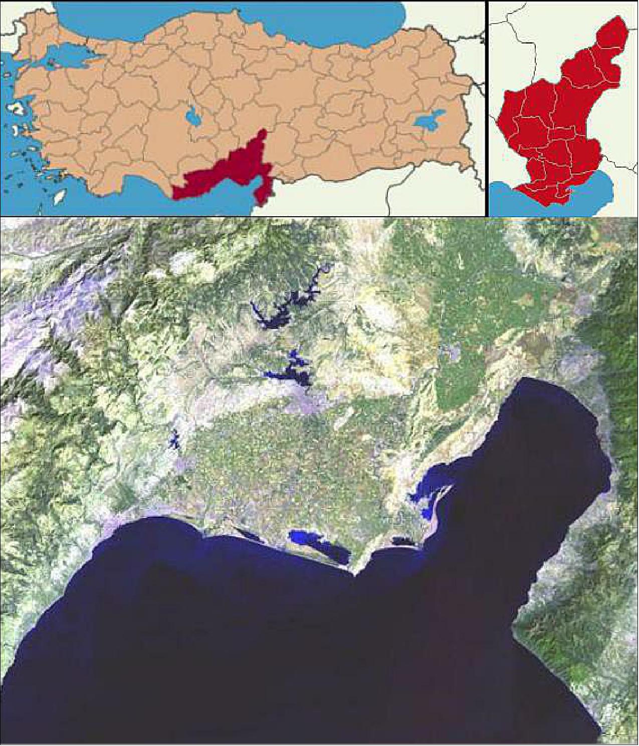
• July 2016: Soil salinity is one of the most important problems affecting many areas of the world. Saline soils present in agricultural areas reduce the annual yields of most crops. This research deals with the soil salinity mapping of the Seyhan plate of Adana district in Turkey from the years 2009 to 2010, using remote sensing technology. In the analysis, multitemporal data acquired from Landsat-7 ETM+ satellite in four different dates (19 April 2009, 12 October 2009, 21 March 2010, 31 October 2010) are used. 42)
- The main objectives of this study are: (i) to understand the spectral reflectance characteristics of saline soil in the Seyhan plate, (ii) to explore the potential of Landsat imagery to detect and map the soil salinity over the study area, (iii) to analyze the correlation between field measurements and Landsat imagery, and (iv) to produce the soil salinity map according to high, moderate and low saline content.
- Study area: Çukurova is a district in south central of Turkey covering the provinces of Adana and Mersin (Figure 38). It is located in the coordinates of 37º02'52'' North latitudes and 35º17'54'' East longitudes. The total area of the Çukurova is about 38,000 km2, Turkey’s biggest delta plain with a large stretch of flat and fertile land, which is among the most agriculturally productive areas of the world. The climate is relatively mild and humid in the winter months and the alluvial soils make the area highly suitable for agriculture. The Akarsu irrigation basin and the Seyhan plate are located in the Çukurova plain.
- In this study, the Landsat-7 ETM+ satellite images with 30 m resolution were used. The images were georectified to a UTM (Universal Transverse Mercator) coordinate system, using WGS (World Geodetic System) 1984 datum, assigned to north UTM zone 36 and Path 175 Row 34, 35. The most compatible and close dates were selected according to the dates of field work not to have any problems like seasonal changes. The dates of satellite images used are given in the Table 6.
Date of field measurements | Date of satellite pass |
02-05-2009 | 19-04-2009 |
04-10-2009 | 12-10-2009 |
04-10-2010 | 31-10-2010 |
24-03-2010 | 21-03-2010 |
- Ground truth measurements: Fieldwork performed by Cukurova University, Remote Sensing and GIS group in May 2009, October 2009, October 2010 and March 2010, were used in the analysis. In these periods, different numbers of soil samples and soil EC (Electrical Conductivity ) were collected by using the EM-38 device. As a total, 688, 269,153, and 27 samples were collected in the periods of 12-Oct-2009, 31-Oct-2010, 19- Apr-2009 and 21-Mar-2010, respectively. The dataset consists of four Landsat images belonging to the years 2009 and 2010 winter and summer cropping seasons; hence it is possible to evaluate the soil salinity conditions in both seasonal and annual periods.
- As a first step, preprocessing of Landsat images is applied. Several salinity indices such as NDSI (Normalized Difference Salinity Index), BI (Brightness Index) and SI (Salinity Index) are used besides some vegetation indices such as NDVI (Normalized Difference Vegetation Index), RVI (Ratio Vegetation Index), SAVI (Soil Adjusted Vegetation Index) and EVI (Enhanced Vegetation Index) for the soil salinity mapping of the study area.
Results (Ref. 42):
- As a first approach, simple linear regression technique was applied to each individual bands and low correlation (r2: - 30.89% to 20.02%) was observed. As a second approach, the multiple linear regression was applied to all bands of satellite images. Among all different band combinations tested, the correlation of 18 sampled points of March 21, 2010 with EC measurements, showed the highest correlation (78.40%) due to near simultaneous acquisition of the satellite data (3 days).
- After the correlation analysis, the satellite data showing the highest correlation (March 21, 2010) were chosen to map the soil salinity in the area As observed, the highest saline soils in the study area are taking place in the region covering reeds due to the presence of high amount of salt in the lake. Besides, the other parts of the Seyhan plate are being affected by medium to low soil salinity and the salt is mostly accumulated in the lower part of the study area.
- As a final step, the percentages of the salt-affected fields in the study area were evaluated. taking into two major fields into account, it was seen that bare soil fields are rather more influenced by salinization than the wheat fields due to having direct interaction.
The following list is a summary of the main conclusions, drawn from this study:
- The compatibility between the satellite data and the field data; the more simultaneous satellite data and field measurements are used, the better a correlation can be observed.
- Radiometric quality of Landsat-7 ETM+data: the missed lines can make it difficult to get the exact value of a pixel or visually affect the image interpretation. Although the scan line error of Landsat-7 ETM+ can be corrected using the available remote sensing software, the original values are modified.
- Spatial resolution of Landsat-7 satellite 30 m data: the higher resolution makes the sampling easier in the image data.
- Spectral resolution of Landsat-7 satellite data: Hyperspectral sensors can be a better solution, since they capture a large amount of narrow bands.
As a continuation of this study, it is planned to test the other multispectral/hyperspectral sensor data in the same area to evaluate the effectiveness of the different spectral/spatial resolutions on the salinity mapping in the future.
• In November 2015, Landsat-7 still acquires geometrically and radiometrically accurate data worldwide, and methods have been established that allow users to fill the data gaps. 43)
- Landsat data support a vast range of applications in areas such as global change research, agriculture, forestry, geology, land cover mapping, resource management, water, and coastal studies. Specific environmental monitoring activities such as deforestation research, volcanic flow studies, and understanding the effects of natural disasters all benefit from the availability of Landsat data. In recent years, Landsat data have also been used to track oil spills and to monitor mine waste pollution. Table 7 lists Landsat bands and describes the use of each band to help users determine the best bands to use in data analysis.
Band name | LS8 | LS7 (ETM+) | LS4-5 (TM) | LS4-5 (MSS) | LS1-3 (MSS) | Description of use |
Coastal/Aerosol | Band 1 | - | - | - | - | Coastal areas and shallow water observations; aerosol, dust, smoke detection studies |
B (blue) | Band 2 | Band 1 | Band 1 | - | - | Bathymetric mapping; soil/vegetation discrimination, forest type mapping, and identifying manmade features |
G (green) | Band 3 | Band 2 | Band 2 | Band 1 | Band 4 | Peak vegetation; plant vigor assessments |
R (Red) | Band 4 | Band 3 | Band 3 | Band 2 | Band 5 | Vegetation type identification; soils and urban features |
NIR (Near Infrared) | Band 5 | Band 4 | Band 4 | Band 3 | Band 6 | Vegetation detection and analysis; shoreline mapping and biomass content |
SWIR1 (Shortwave Infrared-1) | Band 6 | Band 5 | Band 5 | - | - | Vegetation moisture content/drought analysis; burned and fire-affected areas; detection of active fires |
SWIR2 (Shortwave Infrared-2) | Band 7 | Band 7 | Band 7 | - | - | Additional detection of active fires (especially at night); plant moisture/drought analysis |
PAN (Panchromatic) | Band 8 | Band 8 | - | - | - | Sharpening multispectral imagery to higher resolution |
Cirrus | Band 9 | - | - | - | - | Cirrus cloud detection |
TIR (Thermal Infrared) | Band 10 | Band 6 | Band 6 | - | - | Ground temperature mapping and soil moisture estimations |
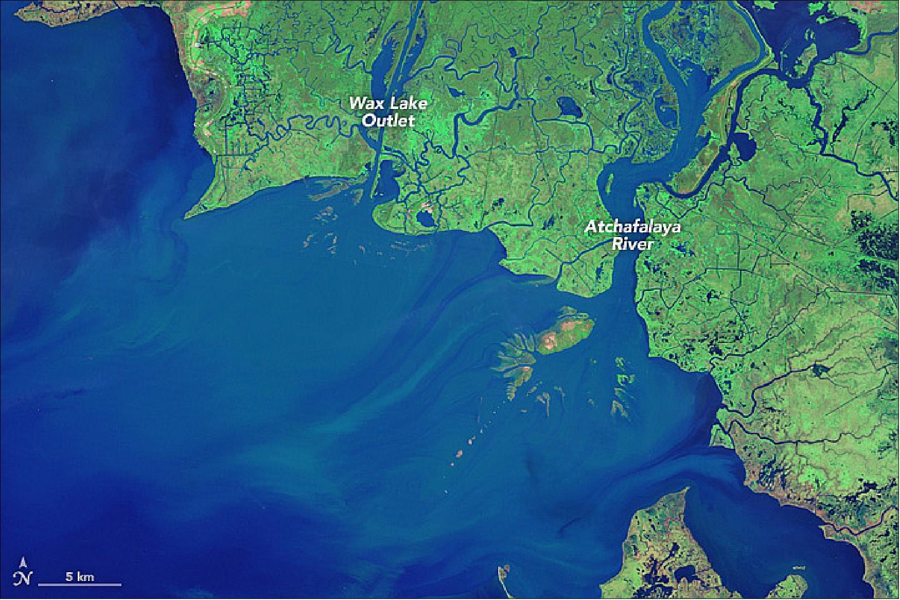
• October 12, 2015: The delta plain of the Mississippi River is disappearing. The lobe-shaped arc of coastal land from the Chandeleur Islands in eastern Louisiana to the Sabine River loses a football field’s worth of land every hour. Put another way, the delta has shrunk by nearly 5,000 km2 over the past 80 years. That’s as if most of Delaware had sunk into the sea. 44)
- Though land losses are widely distributed across the 300 km wide coastal plain of Louisiana, Atchafalaya Bay stands as a notable exception. In a swampy area south of Morgan City, new land is forming at the mouths of the Wax Lake Outlet and the Atchafalaya River. Wax Lake Outlet is an artificial channel that diverts some of the river’s flow into the bay about 16 km west of where the main river empties.
- This series of false-color satellite images chronicles the growth of the two deltas between 1984 and 2015. All of the images were acquired by instruments on Landsat satellites: the Thematic Mapper on Landsat 5, the Enhanced Thematic Mapper Plus on Landsat 7, and the Operational Land Imager on Landsat 8. A combination of shortwave infrared, near infrared, and green light was used to accentuate differences between land and water. Water appears dark blue; vegetation is green; bare ground is pink. All of the images were acquired in autumn, when river discharge tends to be low.
- Note: Only 2 images of the series of 17 images of the study are shown here (the first, Figure 40 and the last, Figure 41).
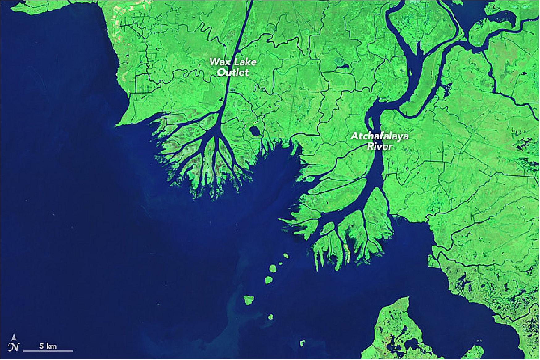
- Both deltas are being built by sediment carried by the Atchafalaya River. The Atchafalaya is a distributary of the Mississippi River, connecting to the “Big Muddy” in south central Louisiana near Simmesport. Studies of the geologic history of the meandering Mississippi have shown that—if left to nature—most of the river’s water would eventually flow down the Atchafalaya. But the Old River Control Structure, built in the 1960s by the U.S. Army Corps of Engineers, ensures that only 30 percent of the Mississippi flows into the Atchafalaya River, while the rest of the keeps moving toward Baton Rouge and New Orleans.
- Even the Atchafalaya’s flow has been sub-divided. In 1941, the Army Corps opened the Wax Lake Outlet, a dredged channel designed to reduce the severity of floods in Morgan City. About 40 percent of the Atchafalaya’s discharge gets channeled through the Wax Lake Outlet.
- Even with the reduced flow, the Atchafalaya carries enough sediment to build land. While geologists first noticed mud deposits building up in Atchafalaya Bay in the 1950s, new land first rose above the water line in 1973 after a severe flood. Since then, both deltas have grown considerably. According to one estimate by scientists from Louisiana State University (LSU), the Atchafalaya and Wax Lake Outlet deltas have combined to grow by 2.8 km2 per year.
- The rate of growth has varied considerably, mainly due to the timing of major floods and hurricanes. Floods transport large volumes of extra sediment to Atchafalaya Bay, while hurricanes redistribute sediment within the bay and transport it offshore into deeper waters. Hurricanes also destroy coastal vegetation that would otherwise protect land from erosion.
- The two deltas added a combined 34 km2 of land between 1989 and 1995, for instance, but lost 2 km2 between 1999–2004, according to the LSU team. The land loss coincided with a period when hurricanes Allison, Isidore, and Lili battered Atchafalaya Bay and there were no major floods to replenish sediments.
- As is typical of deltas in southern Louisiana, the Atchafalaya and Wax Lake Outlet deltas have grown southward into the Gulf of Mexico. While the newer, outer lobes are periodically submerged by the sea and are still free of vegetation, various types of plants—including reeds and willows—colonize the higher elevations of the sandbars. Vegetation is critical to maintaining new land because roots stabilize sediment and prevent erosion.
- The Atchafalaya delta has grown at a faster rate than its neighbor—about 1.6 km2 per year, versus 1.2 km2 per year for the Wax Lake delta. The difference is due to regular dredging and channel widening on the lower Atchafalaya, which delivers extra sediment to its delta. In the sequence of images, the emergence of new dredged islands—which appear pink—is particularly noticeable between 1993 and 1994. Due to the lack of dredging, Wax Lake delta is more natural in character, with a more symmetric, lobate shape.
- So why are the deltas in Atchafalaya Bay growing while the rest of Louisiana’s coastline is retreating? The key reason is that the Atchafalaya delivers sediment to the coast at a pace that allows it to settle into shallow water and to maintain marshes. In contrast, an extensive series of levees keep the Lower Mississippi’s water flowing in a narrow channel that whisks water and sediment past natural floodplains. Instead of building new land along the mouth of the Mississippi, the controlled river sends jets of sediment-rich water directly into the relatively deep waters of the Gulf of Mexico and toward the edge of the continental shelf.
- With sea level rising rapidly due to natural geological processes, climate change, and human activities, predictions for the future of the Mississippi Delta are grim. Even the land gains in Atchafalaya Bay will do little to offset the losses elsewhere, according to geologists. Most scientists expect the Mississippi Delta Plain to lose roughly 5,000 km2 of land over the next 50 years.
- “We are looking carefully at the Wax Lake and Atchafalaya deltas as models for building new land and preserving some of our coastal marshlands,” said Harry Roberts, director of the Coastal Studies Institute at LSU. “If we start diverting significant portions of the water and sediment from the main channel of the Mississippi River into adjacent wetlands, lakes, and bays—as happens now in Atchafalaya Bay—we’ll be taking an important first step toward saving a significant part of Louisiana’s coastal plain.”
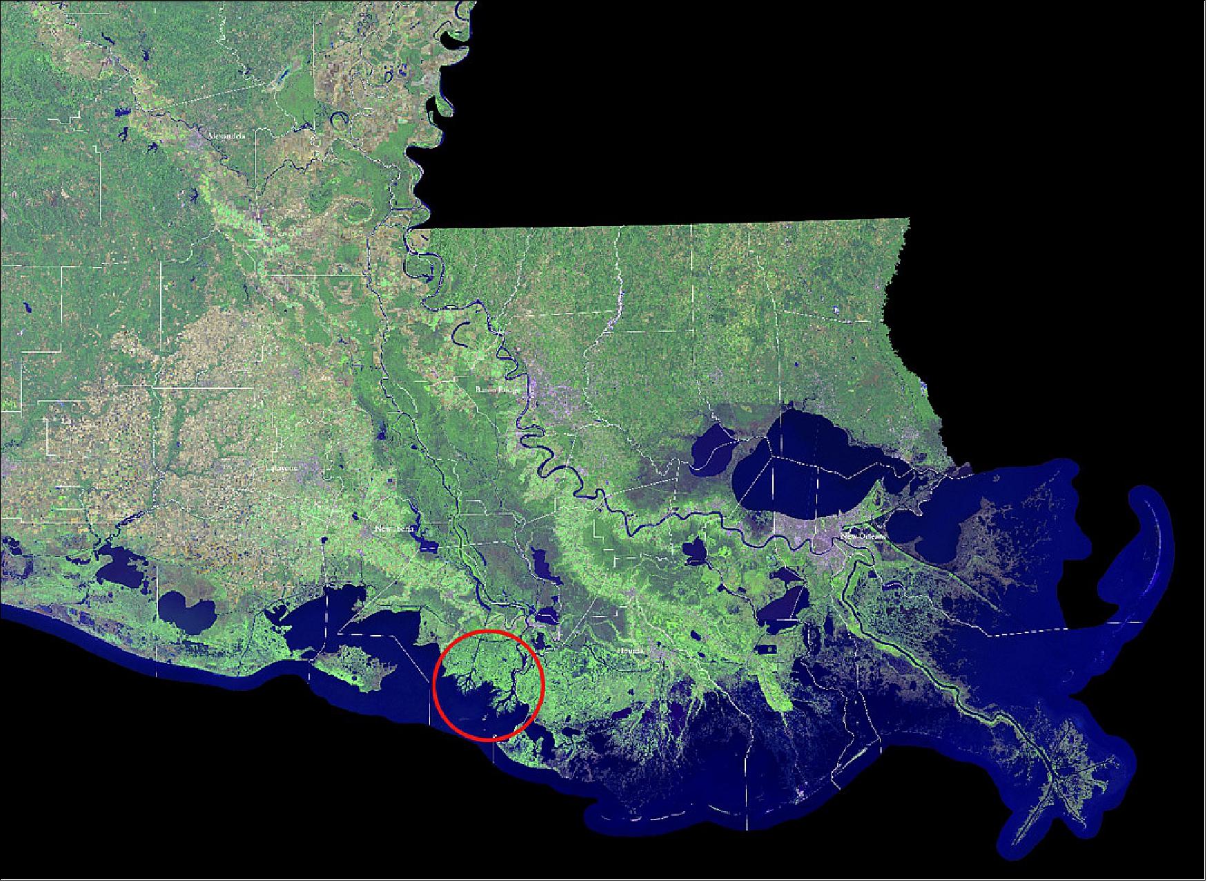
• On April 15, 2015, Landsat-7 was on orbit for 16 years, well past its 5-year design life. A number of spacecraft components are being monitored (e.g., attitude control system, remote telemetry command box, power control unit) but overall, Landsat-7 is acquiring more imagery than at any point in its history (collecting about 475 scenes/day, ~22% of pixels are missing per scene (faulty scan-line corrector). 45) 46)
- There was considerable discussion on the end-of-mission for Landsat-7. Fuel depletion is expected by late 2018, but the imaging life can be extended with reduced orbit maintenance. Preliminary analysis shows that if Landsat-7 is authorized to continue imaging outside of its nominal 10:00 AM equator crossing time window, the mission could be extended until early 2020. At that point, however, the local solar time would be 9:15 AM. The LST (Landsat Science Team) encouraged continued imaging until 2020. As Landsat 5 orbit decayed to an approximate 9:15 AM orbit in the late 1990s, there is precedent for imaging outside the nominal crossing time.
• Landsat-7 is operational in 2015 with the known degradations of the ETM+ instrument, collecting global data.
• On April 2014, the Landsat-7 satellite has now been observing Earth from outer space for 15 years. 47)
• Landsat-7 status on March 3, 2014: The spacecraft continues its science mission. 48)
- Currently, the Landsat-7 archive is providing 1,708,353 scenes of ETM+ data which corresponds to ~ 1,586 TB Raw and L0Ra Data (average scene size of 487 MB). 49)
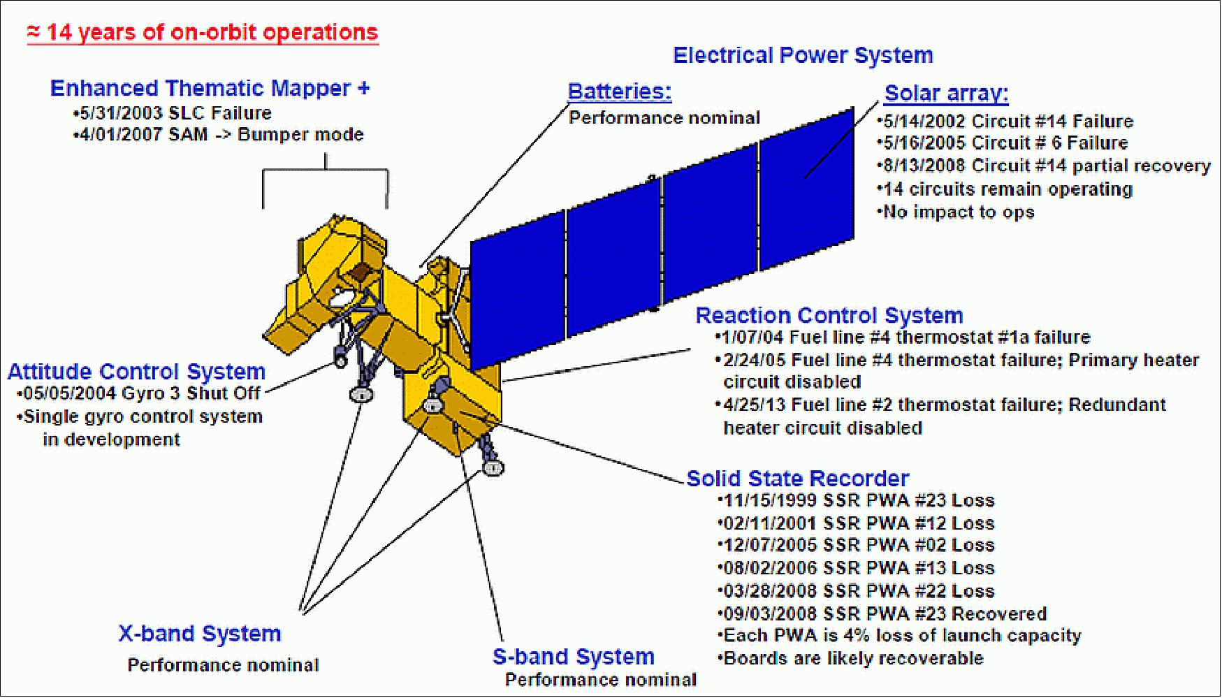
• January 2014: Landsat-7 continues its science mission and based on fuel estimates will continue to do so until at least mid-2016. Landsat-7, while its imagery is slightly degraded due to the scan-line corrector failure, continues to provide global coverage and an 8-repeat cycle for the Landsat Mission when combined with Landsat-8. 50)
• The LS-7 spacecraft is operational in 2013 with the known degradations of the ETM+ instrument, collecting global data. 51)
- Launched on April 15, 1999 with a 5 year design life, the Landsat-7 mission just began its 14th year on-orbit.
- Robust global acquisitions are continuing, collecting nearly 400 scenes a day.
- Fuel-based end-of-life is 2017.
- Successfully completed the underflight with LDCM, collecting all images that LDCM collected for a three day period.
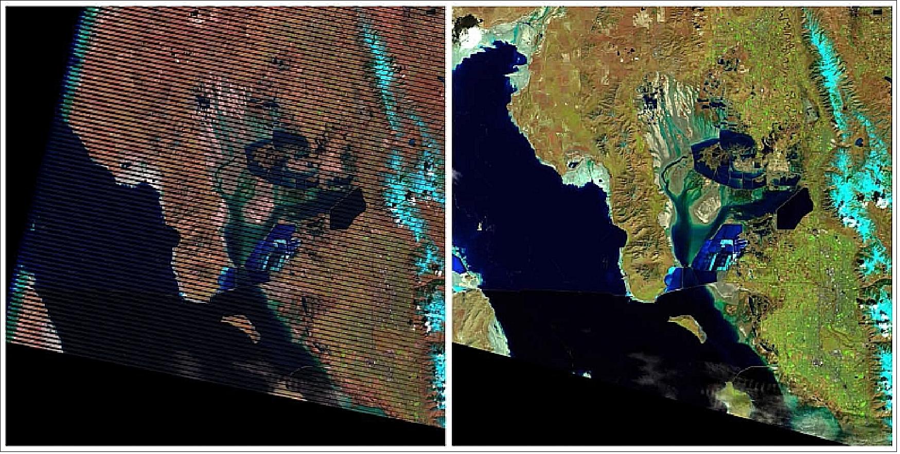
Legend to Figure 44: On March 29-30, 2013, the LDCM was in position under the Landsat 7 satellite. This provided opportunities for near-coincident data collection from both satellites. The images below show a portion of the Great Salt Lake in Utah, and the Dolan Springs, Arizona area, the latter of which is used in Landsat calibration activities. 52)
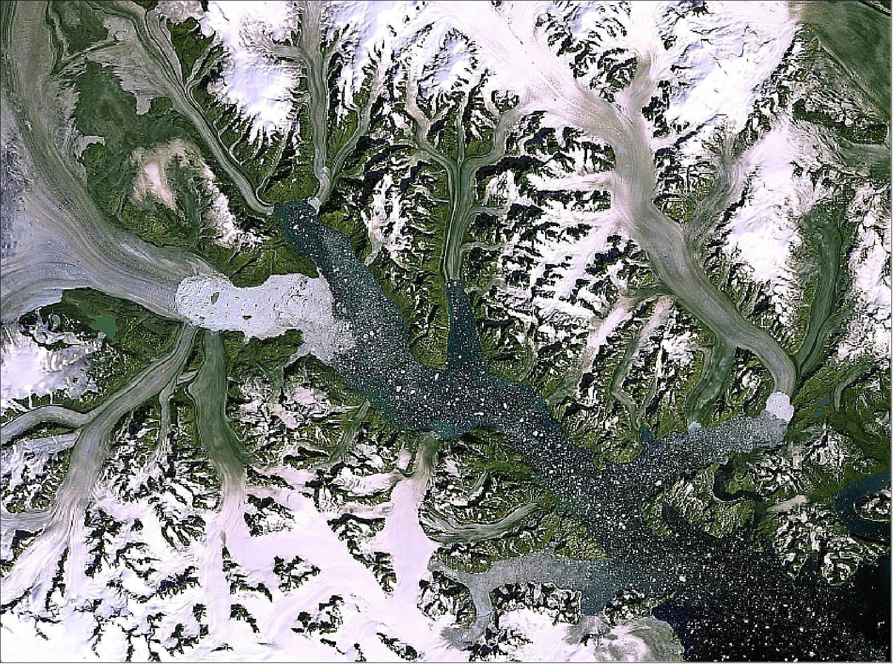
Legend to Figure 45: This image, released on Dec. 21, 2012, shows the largest outlet glacier on Greenland’s east coast, discharging ice into the surrounding oceans. In this image one can see hundreds of icebergs speckling the water. A recent study based on satellite observations revealed that over the past 20 years the ice melting in Greenland and Antarctica has contributed about 11 mm to the global sea-level rise. This image clearly shows the glacier’s calving front, where ice breaks away. Over the years, satellite images have shown that this front has retreated – an indication that the glacier is getting smaller over time.
• On July 23, 2012, the Landsat program marked its 40th anniversary, representing the longest continuous global record of Earth observations from space. Through four decades, Landsat satellites have taken specialized measurements of Earth's continents and surrounding coastal regions, enabling people to study many aspects of our planet and to evaluate the dynamic changes caused by both natural processes and human practices. The long record of Landsat spectral information is a historical archive unmatched in quality, detail, coverage, and length. 54)
The data-rich USGS archive built from the Landsat satellites since 1972, with more than three million images, represents the surface of Earth over a 40-year period, a story of our physical world unparalleled in the history of science.
• The LS-7 spacecraft is operational in 2012 with the known degradations of the ETM+ instrument. 55)
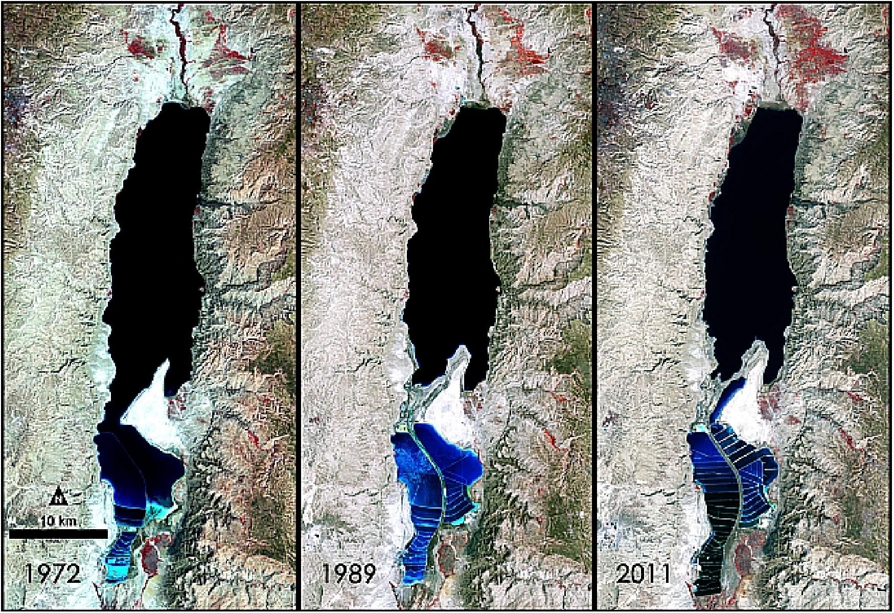
Legend to Figure 46: The 3 Landsat images were captured by the Landsat-1, -4 and -7 satellites. Visible is the Lisan Peninsula (bottom center) that forms a land bridge through the Dead Sea. Deep waters are dark blue, while pale blue shows salt ponds and shallow waters to the south. The pale pink and sand-colored regions are desert lands. Denser vegetation appears bright red. - The expansion of massive salt evaporation projects on the Dead Sea are clearly visible in this time series of images taken by Landsat satellites operated by NASA and the USGS (U.S. Geological Survey). The USGS preserves a 40-year archive of Landsat images that is freely available data over the Internet.
• The LS-7 spacecraft is operational in 2011 (11 years of on-orbit operations). 57)
• LS-7 is operational in 2010 providing image data, however with the known degradations of the ETM+ instrument. Expendable fuel, necessary for stabilizing the orbit and angle of the satellite, will run out in 2012. 58) 59) 60)
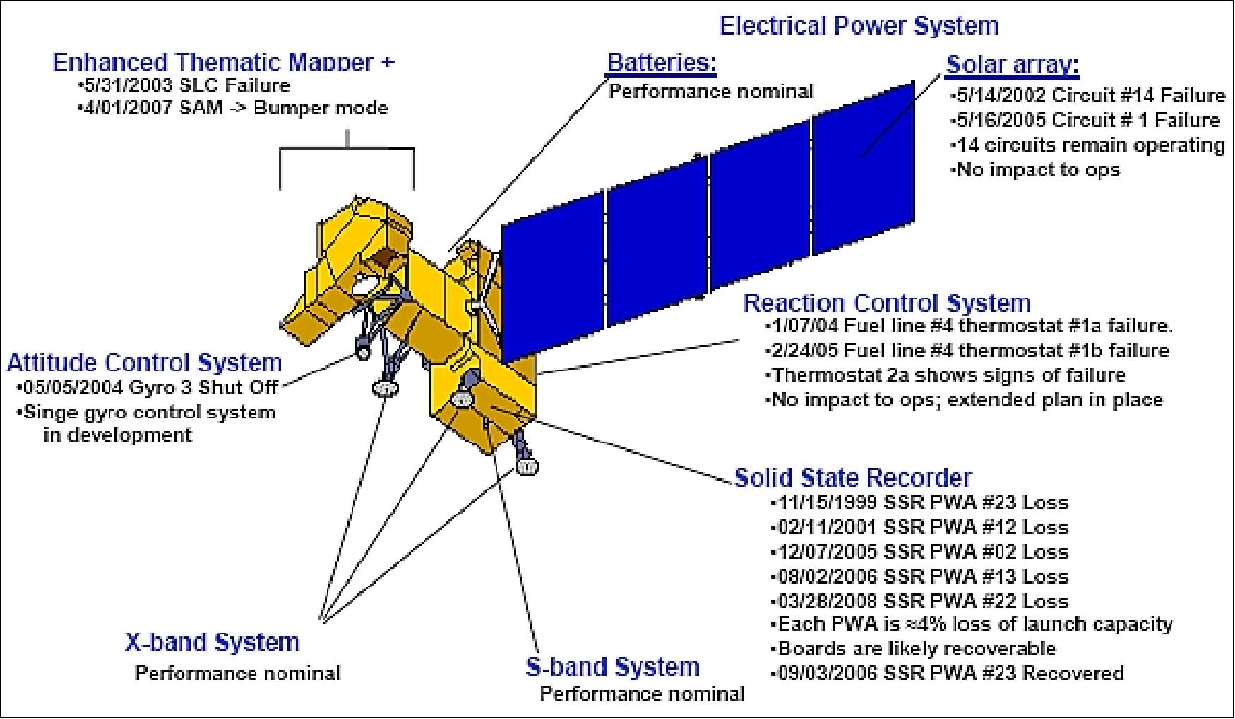
• The Landsat 7 ETM+ instrument is currently operating in SAM (Scan Angle Monitor) mode to control the motion of the scan mirror during imaging. Over time, wear of the scan mirror assembly will cause the instrument to lose the ability to synchronize the calibration shutter with the scan mirror. - Current projections show this to occur between March 2007 and January 2008. As a result, changes to operations and software are necessary to switch the instrument to an alternate mode, known as “bumper mode.” The Landsat-5 Thematic Mapper underwent a similar change in 2002. 61)
• In preparation for this event, on March 3rd and 19th, 2006, the Landsat-7 flight operations team successfully tested bumper mode operation over several geometric calibration sites. Analysis of the preliminary data show the movement of one of the antennas impacts image acquisition, but this error can be corrected by the ground processing system. Additional in-depth research is underway, but this successful bumper mode test is a positive indicator for the continuation of the Landsat-7 mission.
• The Landsat-7 spacecraft and its payload reached the end of its five-year design life on April 15, 2004.
Spacecraft gyros status
The LS-7 project de-powered one of its gyros on May 5, 2004, due to indications of anomalous behavior. The spacecraft has three two-degrees-of-freedom gyros and needs two at any time to maintain attitude control. A risk assessment reported a 40 percent likelihood of another gyro failure by July 2005. A team was assembled to modify the software on board the spacecraft to operate in what is being termed Virtual Gyro (V-Gyro) mode. In this mode, if another gyro fails, the attitude control system would use the remaining gyro, along with existing onboard instrumentation and new control logic, to maintain attitude control.
As of February 1, 2006, the Landsat-7 team developed and uploaded flight software that can act like a ”virtual” gyro -- ready to use if another gyro fails. The enhanced capability was designed, developed, tested, and implemented with no interference to ongoing Landsat-7 operations.
Ground Segment
Landsat-7 data is received and distributed to the user community by USGS (capturing and processing 250 Landsat scenes per day and delivering at least 100 of the scenes to users each day).NASA/GSFC performed on-orbit mission operations until Oct. 1, 2000; after that responsibility for flight operations and LS-7 management was transferred to the USGS/EDC (flight operations, maintenance, and management of all ground data reception, processing, archiving, product generation, and distribution). The operating philosophy changed to the effect that ETM+ data covering the global continental surfaces are being archived in the USA. The ETM+ archive is continually being updated as data become available. This data policy differs from the past (Landsat-4 and -5), where data was only acquired from the S/C on the basis of customer requests. The new archiving policy will substantially increase the amount of data available to the user community. 62) 63) 64)
The Landsat-7 ground system design includes an Image Assessment System (IAS) to provide users with ancillary information needed to generate useful, radiometrically calibrated and geometrically corrected ETM+ digital imagery. Another aspect of the new data handling policy is that ETM+ data will be distributed from the archive in an essentially raw form. Users are responsible for the task of preprocessing their imagery (i.e. radiometric and geometric corrections). The price tag for Landsat-7 imagery is substantially lower than for the commercial products of Landsat-4 and -5.
• In April 2008, the USGS announced to open the Landsat-7 archive providing free access to the entire user community. Previously acquired imagery from Landsat 1 through Landsat 5, is also now available for download at no charge using the same standard processing format. The release schedule is shown in Table 8. 65)
As of early January 2009, over 225,000 scences were downloaded since Oct. 1, 2008. Newly acquired Landsat 7 ETM+ SLC-off and Landsat 5 TM images with less than 40 percent cloud cover are automatically processed and made available for immediate download. Imagery with greater than 40 percent cloud cover can be processed upon request. Once the requested scenes are processed, an email notification is sent to the customer with instructions for downloading. These scenes will then become accessible to all users. 66)
Data | Available over the Internet |
Landsat 7 – all new global acquisitions | July 2008 |
Landsat 7 – all data | September 2008 |
Landsat 5 – all TM data | December 2008 |
Landsat 4 – all TM data | January 2009 |
Landsat 1-5 – all MSS data | January 2009 |
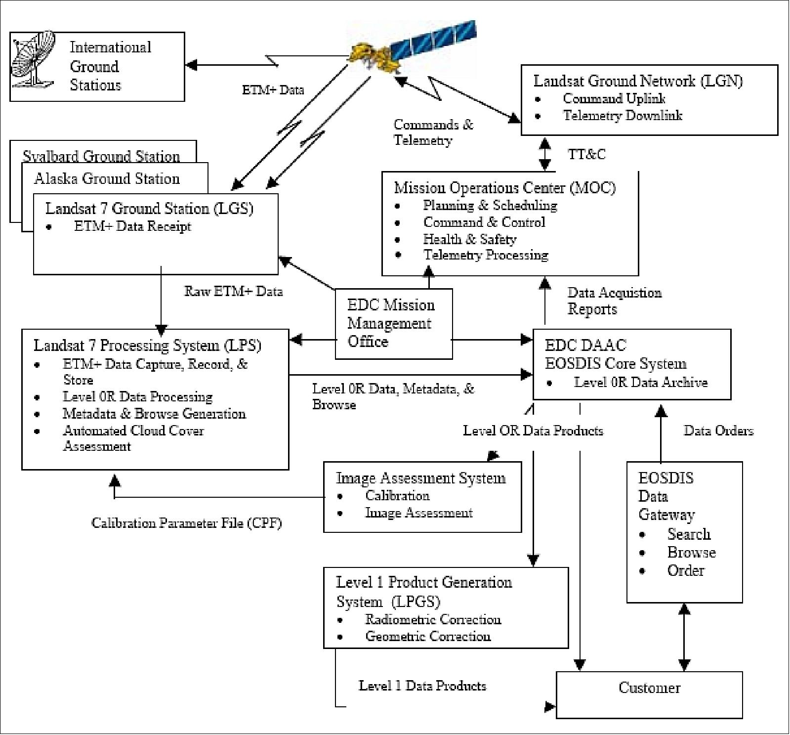
The direct downlink service to a global network of existing Landsat ground stations (in X-band via each of three directional antennas) is maintained. All real-time image data (within view of a licensed ground station) are directly downlinked via the three X-band links. TDRSS may be used for TT&C data relays in S-band (backup). The prime (US) ground receiving station for the Landsat-7 archive is located at the EROS Data Center (EDC) in Sioux Falls, South Dakota. A second (US) reception facility near Fairbanks, AK, acquires coverage of Alaska and international coverage using the onboard recorder. An additional receiving station in Svalbard/Spitzbergen (Norway) provides backup reception. All data received at either Fairbanks or Svalbard is being shipped to EDC for archiving and distribution.
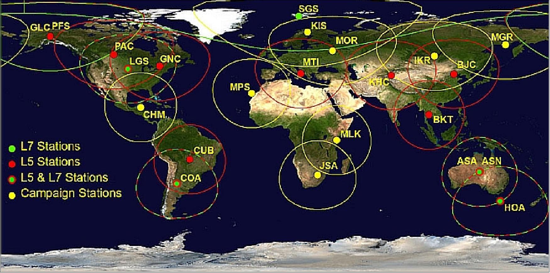
References
1) Special issue on Landsat Sensor Performance Characterization, IEEE Transactions on Geoscience and Remote sensing, Vol. 42, No 12, Dec. 2004
2) “Landsat: A Global Land-Imaging Project,” USGS, URL: http://pubs.usgs.gov
/fs/2010/3026/pdf/FS2010-3026.pdf
3) “Landsat-7 Science Data Handbook,” USGS, URL: http://landsathandbook.gsfc.nasa.gov/
4) K. Dolan, P. Sabelhaus, D. Williams, “Landsat-7 Extending 25 Years of Global Coverage,” Proceedings of Information for Sustainability, 27th International Symposium on Remote Sensing of Environment, Tromsoe, Norway, June 8-12, 1998, pp. 622-625
5) “Landsat-7 Science Data Users Handbook,” URL: http://landsathandbook.gsfc.nasa.gov/payload/
6) B. L. Markham, et al., “Radiometric Calibration of the Landsat-7 Enhanced Thematic Mapper Plus,” Proceedings of IGARSS '94, Volume IV, pp. 2004-2006
7) K. Thome, B. Markham, J. Barker, P. Slater, S. Biggar, “Radiometric Calibration of Landsat,” PE&RS, July 1997, pp. 853-858
8) J. R. Irons, D. L. Williams, B. L. Markham, “Landsat-7 ETM+ on-orbit calibration and data quality assessment,” Proceedings of IGARSS'95, Florence, Italy, July 10-14, 1995, pp. 1573-1575
9) B. L. Markham, D. L. Williams, J. R. Irons, “Landsat Sensor Performance: History and Current Status,” IEEE Transactions on Geoscience and Remote sensing, Vol. 42, No 12, Dec. 2004, pp. 2691-2694
10) D. S. Lee, J. C. Storey, M. J. Choate, R. W. Hayes, “Four Years of Landsat-7 On-Orbit Geometric Calibration and Performance,” IEEE Transactions on Geoscience and Remote sensing, Vol. 42, No 12, Dec. 2004, pp. 2786-2795
11) P. L. Scaramuzza, B. L. Markham, J. A. Basi, E. Kaita, “Landsat-7 ETM+ On-Orbit Reflective-Band Radiometric Correction,” IEEE Transactions on Geoscience and Remote sensing, Vol. 42, No 12, Dec. 2004, pp. 2766-2809
12) J. C. Storey, “Landsat 7 on-orbit modulation transfer function estimation,” Proceedings of SPIE, 'Sensors, Systems, and Next-Generation Satellites,' V, Hiroyuki Fujisada, Joan B. Lurie, Konradin Weber, Editors, Vol. 4540, 2001, URL: http://landsathandbook.gsfc.nasa.gov/pdfs/L7_MTF_Storey_SPIE2001.pdf
13) G. Chander, D. J. Meyer, D. L. Helder, “Cross Calibration of the Landsat-7 ETM+ and EO-1 ALI Sensor;” IEEE Transactions on Geoscience and Remote sensing, Vol. 42, No 12, Dec. 2004, pp. 2821-2831
14) J. G. Masek, M. Honzak, S. N. Goward, P. Liu, E. Pak, “Landsat-7 ETM+ as an observatory for land cover :Initial radiometric and geometric comparisons with Landsat-5 Thematic Mapper,” Remote Sensing of Environment Vol. 78, 2001, pp. 118-130
15) B. L. Markham, J. L. Barker, J. A. Barsi, E. Kaita, K. J. Thome, D. L. Helder, F. D. Palluconi, J. R. Schott, P. Scaramuzza, “Landsat-7 ETM+ Radiometric Stability and Absolute Calibration,” Proceedings of SPIE, 'Sensors, Systems, and Next-Generation Satellites VI,' Hiroyuki Fujisada, Joan B. Lurie, Michelle L. Aten, Konradin Weber, Editors, Vol. 4881, 2003
16) B. Markham, S. Goward, T. Arvidson, J. Barsi, P. Scaramuzza, “Landsat-7 Long-Term Acquisition Plan Radiometry - Evolution Over Time,” PE&RS (Photogrammetric Engineering & Remote Sensing), Vol. 72, Oct. 2006, pp. 1129-1135
17) T. Arvidson, S. Goward, J. Gasch, D. Williams, “Landsat-7 Long-Term Acquisition Plan: Development and Validation,” PE&RS, Vol. 72, Oct. 2006, pp. 1137-1146
18) S. Goward, T. Arvidson, D. Williams, J. Faundeen, J. Irons, S. Franks, “Historical Record of Landsat Global Coverage: Mission Operations, NSLRSDA, and International Cooperator Stations,” PE&RS, Vol. 72, Oct. 2006, pp. 1155-1168
19) Robert Tetrault, “Access and Availability of Resourcesat-1 AWiFS Data for Agriculture,” http://www.pecad.fas.usda.gov/pdfs/2006/RLT_Access_FAS_AgApnsWorkshop_Sept2006_REV20060927.pdf
20) Deanna Archuleta, “Department of the Interior’s Role in Earth Observation,” Proceedings of JACIE 2010 (Joint Agency Commercial Imagery Evaluation) Workshop, Fairfax VA, USA, March 16-18, 2010, URL: http://calval.cr.usgs.gov/JACIE_files/JACIE10/Presentations/TueAM/Archuleta_3-16-10_JACIE.pdf
21) ”Undercutting Sverdrup Glacier,” NASA Earth Observatory, Image of the Day for 26 January 2021, URL: https://earthobservatory.nasa.gov/images/147776/undercutting-sverdrup-glacier
22) ”Counting Trees in Africa’s Drylands,” NASA Earth Observatory, Image of the Day for 7 December 2020, URL: https://earthobservatory.nasa.gov/images/147612/counting-trees-in-africas-drylands
23) Martin Brandt, Compton J. Tucker, Ankit Kariryaa, Kjeld Rasmussen, Christin Abel, Jennifer Small, Jerome Chave, Laura Vang Rasmussen, Pierre Hiernaux, Abdoul Aziz Diouf, Laurent Kergoat, Ole Mertz, Christian Igel, Fabian Gieseke, Johannes Schöning, Sizhuo Li, Katherine Melocik, Jesse Meyer, Scott Sinno, Eric Romero, Erin Glennie, Amandine Montagu, Morgane Dendoncker & Rasmus Fensholt, ”An unexpectedly large count of trees in the West African Sahara and Sahel,” Nature Communications, Volume 587, pp. 78-82, October 2020, https://doi.org/10.1038/s41586-020-2824-5
24) Mitchell K. Hobish, Laura E. P. Rocchio, Darrel Williams, Samuel Goward, ”The Living Legacy of Landsat 7: Still Going Strong after 20 Years in Orbit,” NASA, The Earth Observer, July-August 2019, Volume 31, Issue 4, pp: 4-14, URL: https://eospso.nasa.gov/sites/
default/files/eo_pdfs/Jul_Aug_2019_final_color_508_0.pdf
25) Michael A. Wulder, Thomas R. Loveland, David P. Roy, Christopher J. Crawford,Jeffrey G. Masek, Curtis E. Woodcock, Richard G. Allen, Martha C. Anderson,Alan S. Belward, Warren B. Cohen, John Dwyer, Angela Erb, Feng Gao, Patrick Griffiths,Dennis Helder, Txomin Hermosilla, James D. Hipple, Patrick Hostert, M. Joseph Hughes,Justin Huntington, David M. Johnson, Robert Kennedy, Ayse Kilic, Zhan Li, Leo Lymburner,Joel McCorkel, Nima Pahlevan, Theodore A. Scambos, Crystal Schaaf, John R. Schott,Yongwei Sheng, James Storey, Eric Vermote, James Vogelmann, Joanne C. White,Randolph H. Wynne, Zhe Zhu, ”Current status of Landsat program, science, and applications,” Remote Sensing of Environment, Volume 225, May 2019, Pages 127-147, https://doi.org/10.1016/j.rse.2019.02.015 , URL: https://reader.elsevier.com/reader/sd/pii/S0034425719300707?
token=A77033BD9D286A27CDBD7B3B9ED6D2C296CA379CB
2C3105DEFB6C55AB7A3448BACC4594FCEF5663E0D95F416A8F2A75A
26) For more information on NAFD, visit: https://web.archive.org/web/20201022203536/https://landsat.gsfc.nasa.gov/watching-a-quarter-century-of-north-american-forest-dynamics-with-landsat/
27) https://sspd.gsfc.nasa.gov/restore-L.html
28) https://web.archive.org/web/20201030010448/https://landsat.gsfc.nasa.gov/how_landsat_helps/
29) ”Mapping the Land Between the Tides,” NASA Earth Observatory, 2 July 2019, URL: https://earthobservatory.nasa.gov/images/145237/mapping-the-land-between-the-tides?src=eoa-iotd
30) ”The Urbanization of Ulaanbaatar,” NASA Earth Observatory, 4 June 2019, URL: https://earthobservatory.nasa.gov/images/145125/the-urbanization-of-ulaanbaatar?src=eoa-iotd
31) ”KBRwyle Awarded $19M to Perform Flight Ops for USGS Satellite That Fights World Hunger, Helps Earth Flourish,” PR Newswire, 21 February 2019, URL: https://www.prnewswire.com/news-releases/
kbrwyle-awarded-19m-to-perform-flight-ops-for-usgs-satellite-
that-fights-world-hunger-helps-earth-flourish-300799280.html
32) ”Daily Operations of Landsat 7,” USGS, Published on Jul 18, 2018, URL: https://www.youtube.com
/watch?v=OGTbWK06FX4&feature=youtu.be
33) ”Glacier Retreat at Cook Ice Cap,” NASA Earth Observatory, 27 April 2018, URL: https://earthobservatory.nasa.gov/IOTD/view.php?id=92059&src=eoa-iotd
34) ”Peru’s Newest National Park,” NASA Earth Observatory, 22 March 2018, URL: https://earthobservatory.nasa.gov/IOTD/view.php?id=91871
35) ”The Spread of Mangroves in Senegal,” NASA Earth Observatory, 21 march 2018, URL: https://earthobservatory.nasa.gov/IOTD/view.php?id=91867
36) ”September 14, 2017 – Landsat 7 Anomaly Resolution,” USGS, URL: https://www.usgs.gov/landsat-missions/september-14-2017-landsat-7-anomaly-resolution
37) ”Fire Scars the Okefenokee,” NASA Earth Observatory, May 11, 2017, URL: https://earthobservatory.nasa.gov/IOTD/view.php?id=90214&src=iotdrss
38) ”Cambodia’s Forests Are Disappearing,” NASA Earth Observatory, Jan. 10, 2017, URL: http://earthobservatory.nasa.gov/IOTD/view.php?id=89413
39) Todd A. Schroeder, Thomas R. Loveland, Michael A. Wulder, James R. Irons, ”Landsat Science Team: 2016 Summer Meeting Summary,” The Earth Observer, Volume 28, Issue 6, November-December 2016, pp: 45-50, URL: https://eospso.nasa.gov/sites/default/files/eo_pdfs/Nov-Dec%202016%20color%20508.pdf
40) ”NASA’s Restore-L Mission to Refuel Landsat-7, Demonstrate Crosscutting Technologies,” NASA Technology, June 23, 2016, URL: https://www.nasa.gov/feature/
nasa-s-restore-l-mission-to-refuel-landsat-7-demonstrate-crosscutting-technologies
41) ”Celebrating 50 years of Landsat Vision,” USGS, Sept. 21, 1966, URL: http://landsat.usgs.gov
/project-eros-idea-worked.php
42) A. Azabdaftari , F. Sunar, ”Soil salinity mapping using multitemporal Landsat data,” Proceedings of the XXIII ISPRS ((International Society for Photogrammetry and Remote Sensing) Congress, Prague, Czech Republic, July 12-19, 2016, doi:10.5194/isprsarchives-XLI-B7-3-2016, URL: http://www.int-arch-photogramm-remote-sens-spatial-inf-sci.net/XLI-B7/3/2016/isprs-archives-XLI-B7-3-2016.pdf
43) Landsat—Earth Observation Satellites, USGS, Nov. 2015, URL: http://pubs.usgs.gov/fs/2015/3081/fs20153081.pdf
44) Adam Voiland, ”Growing Deltas in Atchafalaya Bay,” NASA Earth Observatory, Oct. 12, 2015, URL: http://earthobservatory.nasa.gov/Features/WorldOfChange/wax_lake.php
45) Guy Thayer, “Landsat-7 status,“ in 'Landsat Science Team Meeting: Winter 2015,' The Earth Observer, May-June 2015, Volume 27, Issue 3, p. 20, URL: http://eospso.nasa.gov/sites/default/files/eo_pdfs/May_Jun_2015_color_508.pdf
46) Tim Newman, “Land Remote Sensing Program Update,” USGS, March 18, 2015, URL: https://www.fgdc.gov/ngac/meetings/march-2015/landsat-program-update-ngac-march-2015.pdf
47) John Campbell, “Space Veteran Landsat 7 Marks 15 Years of Observing Earth,” USGS, April 15, 2014, URL: http://www.usgs.gov/blogs/features/usgs_top_story/
space-veteran-landsat-7-marks-15-years-of-observing-earth/
48) Jenn Sabers Lacey, “USGS EROS Center - 40 Years of Service to our Plnat,” Proceedings of JACIE 2014 (Joint Agency Commercial Imagery Evaluation) Workshop, Louisville, Kentucky, USA, March 26-28, 2014, URL: https://calval.cr.usgs.gov/wordpress/wp-content/
uploads/J-Lacey-ASPRS-JACIE-Landsat-March-26-2014-Final1.pdf
49) Jenn Sabers Lacey, “USGS EROS Center - 40 Years of Service to our Plnat,” Proceedings of JACIE 2014 (Joint Agency Commercial Imagery Evaluation) Workshop, Louisville, Kentucky, USA, March 26-28, 2014, URL: https://calval.cr.usgs.gov/wordpress/wp-content/
uploads/J-Lacey-ASPRS-JACIE-Landsat-March-26-2014-Final1.pdf
50) Information provided by James M. Lacasse of USGS Climate and Land Use Change, Sioux Falls, S.D., USA
51) Tom Holm, “Landsat: Building a Future on 40 Years of Success - Status: Landsat 7,” 12th Annual JACIE (Joint Agency Commercial Imagery Evaluation) Workshop , St. Louis, MO, USA, April 16-18, 2013, URL: http://calval.cr.usgs.gov/wordpress/wp-content/uploads/JACIE-LDCM-Status-and-Overview-v4.pdf
52) “LDCM Underfly with Landsat 7,” USGS, March 29, 2013, URL: http://landsat.usgs.gov/LDCM_Underfly_with_Landsat_7.php
53) http://www.esa.int/Our_Activities/Observing_the_Earth/Earth_from_Space_Water_and_ice
54) Joel N. Shurkin, “Landsat Looks and Sees,” Space Daily, July 23, 2012, URL: http://www.spacedaily.com/reports/Landsat_Looks_and_Sees_999.html
56) Aries Keck, “NASA Sees New Salt in an Ancient Sea,” Space Daily, April 11, 2012, URL: http://www.spacedaily.com/reports/NASA_Sees_New_Salt_in_an_Ancient_Sea_999.html
57) Kristi Kline, Rachel Headley, “Landsat Project StatusLandsat,” Proceedings of the Landsat Science Team Meeting, Mesa, AZ, USA, March 1-3, 2011, URL: http://landsat.usgs.gov
/documents/Kline%20-%20Landsat%20Status%20-%20LST%203-2011.pdf
58) Information provided by Ronald E. Beck of USGS
59) Thomas Kalvelage, “Landsat Project Status, Landsat Science Team Meeting,” Jan. 19-21, 2010, Mountain View, CA, USA, URL: http://landsat.usgs.gov/documents/
Jan_2010_ScienceTeamMeeting_LandsatOverview_TomK_final_Jan19.pdf
60) “Landsat Science Team Meetings,” URL: http://landsat.usgs.gov/science_LST_Team_Meetings.php
61) J. A. Barsi, B. L. Markham, D. L. Helder, G. Chander, “Radiometric calibration status of Landsat-7 and Landsat-5,” Proceedings of. SPIE, Vol. 6744, Florence, Italy, Sept. 17-20, 2007, URL: http://landsat.gsfc.nasa.gov/pdf_archive/publications/SPIE07_LandsatRadiometry.pdf
62) J. R. Irons, D. L. Williams, B. L. Markham, “Landsat-7 ETM+ On-Orbit Calibration and Data Quality Assessment,” Proceedings IGARSS '95, Vol. II, pp. 1573-1575
63) W. C. Draeger, T. M. Holm, D. T. Lauer, R. J. Thompson, “The Availability of Landsat Data: Past, Present and Future,” PE&RS, July 1997, pp. 869-875
64) R. A. Williamson, “The Landsat Legacy: Remote Sensing Policy and the Development of Commercial Remote Sensing,” PE&RS, July 1997, pp. 877-885
65) “Imagery for Everyone -- Timeline Set to Release Entire USGS Landsat Archive at No Charge,” April 21, 2008, USGS, URL: http://landsat.usgs.gov/documents/USGS_Landsat_Imagery_Release.pdf
66) http://landsat.usgs.gov/mission_headlines2009.php
67) “International Ground Station (IGS) Network,” USGS, URL: http://landsat.usgs.gov/about_ground_stations.php
68) Landsat 7 Data Acquired at a Lower Orbit Now Available | U.S. Geological Survey. (n.d.). www.usgs.gov. Retrieved October 31, 2022, URL: https://www.usgs.gov/landsat-missions/news/landsat-7-data-acquired-lower-orbit-now-available
The information compiled and edited in this article was provided by Herbert J. Kramer from his documentation of: ”Observation of the Earth and Its Environment: Survey of Missions and Sensors” (Springer Verlag) as well as many other sources after the publication of the 4th edition in 2002. - Comments and corrections to this article are always welcome for further updates (eoportal@symbios.space).
Spacecraft Launch Sensor Complement Mission Status Ground Segment References Back to top