Jason-3 Altimetry Mission
EO
Atmosphere
Ocean
NASA
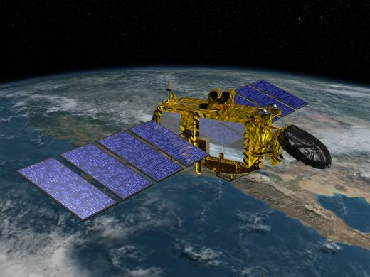
Launched in January 2016, Jason-3 is the follow-on altimetry mission of Jason-2/OSTM (Ocean Surface Topography Mission) developed and led collaboratively by NOAA (National Oceanic and Atmospheric Administration), EUMETSAT (European Organisation for the Exploitation of Meteorological Satellites), CNES (Centre national d'études spatiales) and National Aeronautics and Space Administration (NASA). Its objective is to provide continuity to the Poseidon/TOPEX (Ocean Topography Experiment), Jason-1 and Jason-2 missions which support applications related to extreme weather events, operational oceanography, climate and forecasting. The mission has been extended past its three year nominal lifetime and is operational as of August 2022.
Quick facts
Overview
| Mission type | EO |
| Agency | NASA, CNES, NOAA, EUMETSAT |
| Mission status | Operational (extended) |
| Launch date | 17 Jan 2016 |
| Measurement domain | Atmosphere, Ocean, Land, Gravity and Magnetic Fields |
| Measurement category | Gravity, Magnetic and Geodynamic measurements, Atmospheric Humidity Fields, Landscape topography, Ocean topography/currents, Ocean surface winds, Ocean wave height and spectrum |
| Measurement detailed | Atmospheric specific humidity (column/profile), Land surface topography, Wind speed over sea surface (horizontal), Significant wave height, Geoid, Sea level, Ocean dynamic topography, Gravity field |
| Instruments | LRA, AMR, GPSP, POSEIDON-3B Altimeter, DGXX-S |
| Instrument type | Precision orbit, Imaging multi-spectral radiometers (passive microwave), Radar altimeters |
| CEOS EO Handbook | See Jason-3 Altimetry Mission summary |
Summary
Mission Capabilities
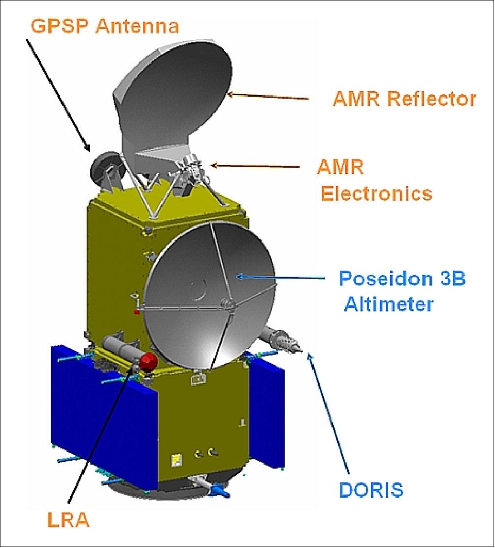
Jason-3 carries five instruments onboard: Poseidon-3B, Advanced Microwave Radiometer-2 (AMR-2), Global Positioning System Payload (GPSP), Doppler Orbitography and Radiopositioning Integrated by Satellite (DORIS) and a Laser Retro-reflector Array (LRA). Funded by EUMETSAT and built by Thales Athenia Space (TAS) (Poseidon-2 heritage), Poseidon-3B is a nadir-looking radar altimeter that serves as the primary instrument in the mission. Its objective is to map the topography of the sea surface for calculating ocean surface current velocity and to measure ocean wave height and wind speed. AMR-2 is funded by NOAA and provided by NASA with the aim to measure the altimeter signal path delay due to tropospheric water vapour. Improving upon the previous generation flown onboard Jason-2, DORIS is funded by EUMETSAT and supplied by CNES to keep permanent track of the satellite’s precise position through the use of global orbitography beacons. GPSP also tracks the satellite’s trajectory continuously through triangulation and is funded by NOAA and supplied by NASA. LRA is a NASA instrument which provides a reference target for satellite laser ranging measurements.
In addition to the sensors, Jason-3 carries a Joint Radiation Experiment (JRE) consisting of CARMEN (ChaRacterization and Modeling of ENvironment) and a Light Particle Telescope (LPT).
Performance Specifications
The objectives of the Jason-3 mission require a global sea surface height measurement to an accuracy of less than 4 cm every 10 days to determine ocean circulation, climate change and sea level rise. It also needs high precision ocean topography measurements beyond those provided by preceding missions. It utilises nadir-only scanning with sampling at 30 km intervals along the track.
Jason-3 undergoes a circular non-sun-synchronous orbit at an altitude of 1336 km and an inclination of 66°. It has a period of approximately two hours and completes a 9.9 day repeat cycle.
Hardware Components
Alike to its predecessor, Jason-3 employs the three-axis stabilised and nadir pointing Proteus bus of CNES/TAS, maintained by reaction wheels and magnetic torque rods. Featuring a mass of 550 kg, it is powered by two solar panels, using a hydrazine propellant system for orbital maintenance. The spacecraft has surpassed its extended design lifetime of five years, remaining operational as of August 2022.
Jason-3 Altimetry Mission
Spacecraft Launch Mission Status Sensor Complement Ground Segment References
Jason-3 is the follow-on altimetry mission of Jason-2 / OSTM (launch June 20, 2008) led by the operational agencies: NOAA, EUMETSAT, and CNES. The objective of the Jason-3 Mission is to provide continuity to the unique accuracy and coverage of the TOPEX/Poseidon, Jason-1 and OSTM/Jason-2 missions in support of operational applications related to extreme weather events and operational oceanography and climate applications and forecasting. 1) 2) 3)
In early February 2010, the EUMETSAT Member States approved the Jason-3 transatlantic program - thus ensuring a continuation of the series of measurements made by the Jason-2 satellite and its predecessors in support of meteorology, operational oceanography and in particular the monitoring of the sea level trend, a key indicator of climate change. The MOU (Memorandum of Understanding) was signed in July 2010. 4) 5) 6) 7) 8)
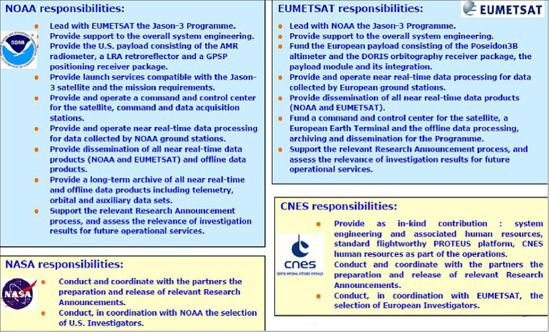
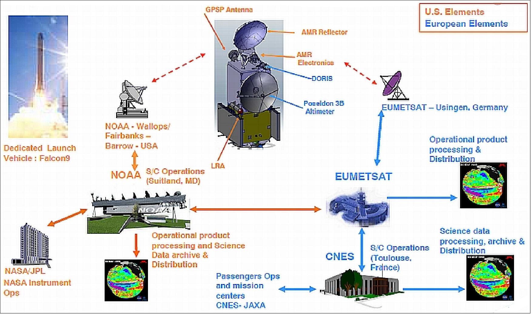
The partnership responsibilities/activities of Jason-3 are distributed in the following way: 9)
• NOAA and EUMETSAT — the operational agencies — are taking the lead
• CNES, the French Space Agency, is making a significant in-kind contribution to the program and will act at the technical level as the system coordinator. This in-kind contribution includes making available the Jason-3 Proteus satellite platform, its facilities and associated human resources.
• NASA, in conjunction with the three other partners (NOAA, EUMETSAT, CNES), will support science team activities. The US contribution to Jason-3 includes the satellite launch, provision of instruments and support to operations.
• Overall, responsibilities sharing has changed, but activities sharing remains almost the same as for Jason-2/OSTM.
Planning for the Jason-CS (Jason-Continuity of Service) mission started in the timeframe 2009/10: The Jason-CS program is the follow-on Reference Mission of Jason-3 spanning the timeframe 2015-2020.
The mission objectives are:
1) Provide continuity of high precision ocean topography measurements beyond TOPEX/Poseidon , JASON-1 and JASON-2
2) Provide an operational mission to enable the continuation of multi-decadal ocean topography measurements
3) The science requirements call for a global sea surface height to an accuracy of < 4 cm every 10 days for determining days, ocean circulation, climate change and sea level rise.
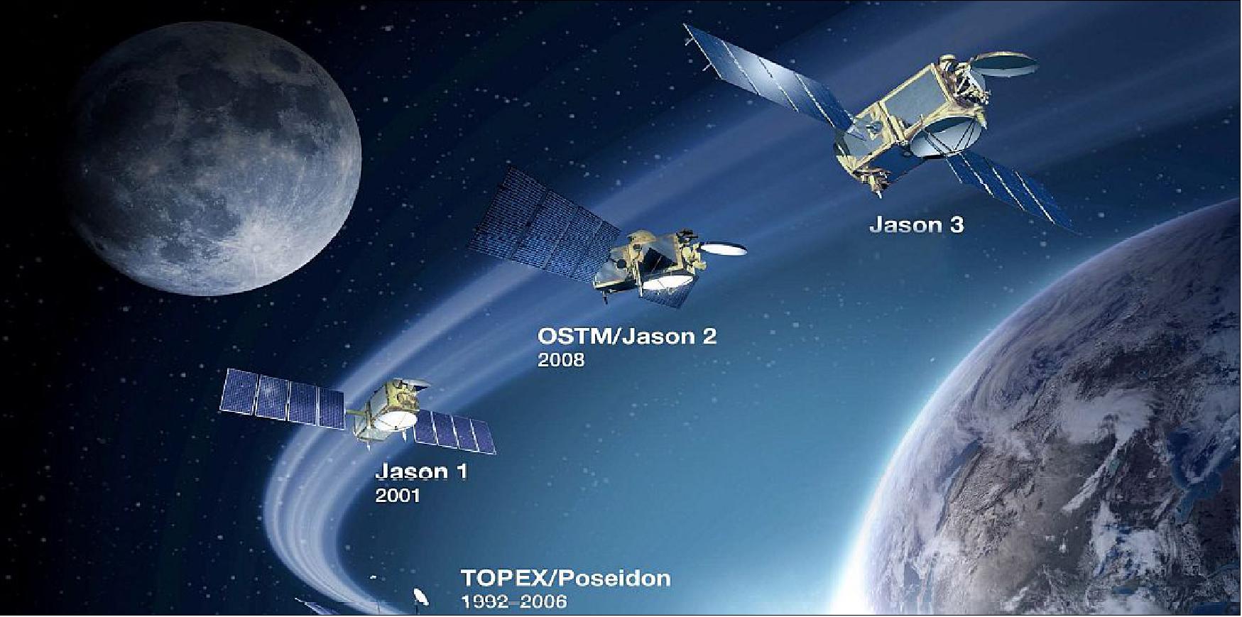
While the Jason-3 mission will continue the core satellite altimetry measurements for physical oceanography - the plans call in addition for the transitioning from research to operational applications of this valuable measurement. Jason-3 builds upon the heritage of the foundational and transitional missions such as SEASAT (1978), GEOSAT (1985), TOPEX/Poseidon (T/P, 1992), Jason-1 (2001) and Jason-2 / OSTM (2008), which have led to the understanding and development of a wide range of oceanographic applications of satellite altimetry. 10)
Fulfilling the goals of moving satellite altimetry onto routine operations will require a close cooperation and coordination of international, multi-agency mission managers, designers, engineers, scientists and operational systems developers.
NOAA and EUMETSAT gained already experience in operating the Jason-2 / OSTM mission. The Jason-3 mission is fully lead by the operational agencies, NOAA and EUMETSAT, with CNES and NASA in supporting roles. 11)
• Ocean-monitoring data exchange between Europe and China: On August 30, 2012, EUMETSAT signed an agreement with NSOAS (National Satellite Ocean Application Service) of China to exchange data from their ocean-monitoring satellites. For EUMETSAT, this applies to data from the missions: Jason-2 and Jason-3 as well as from the MetOp series satellite (ASCAT data). In return, NSOAS will provide EUMETSAT with similar scatterometer and altimetry data from the Chinese HY-1 and HY-2 ocean-color satellites. 12)
Spacecraft
Mission architecture: With a recurring development methodology in mind, the overall mission architecture for Jason-3 is planned to be the same as for Jason-2 / OSTM, taking into account areas of updates due to obsolescence or unavailability.
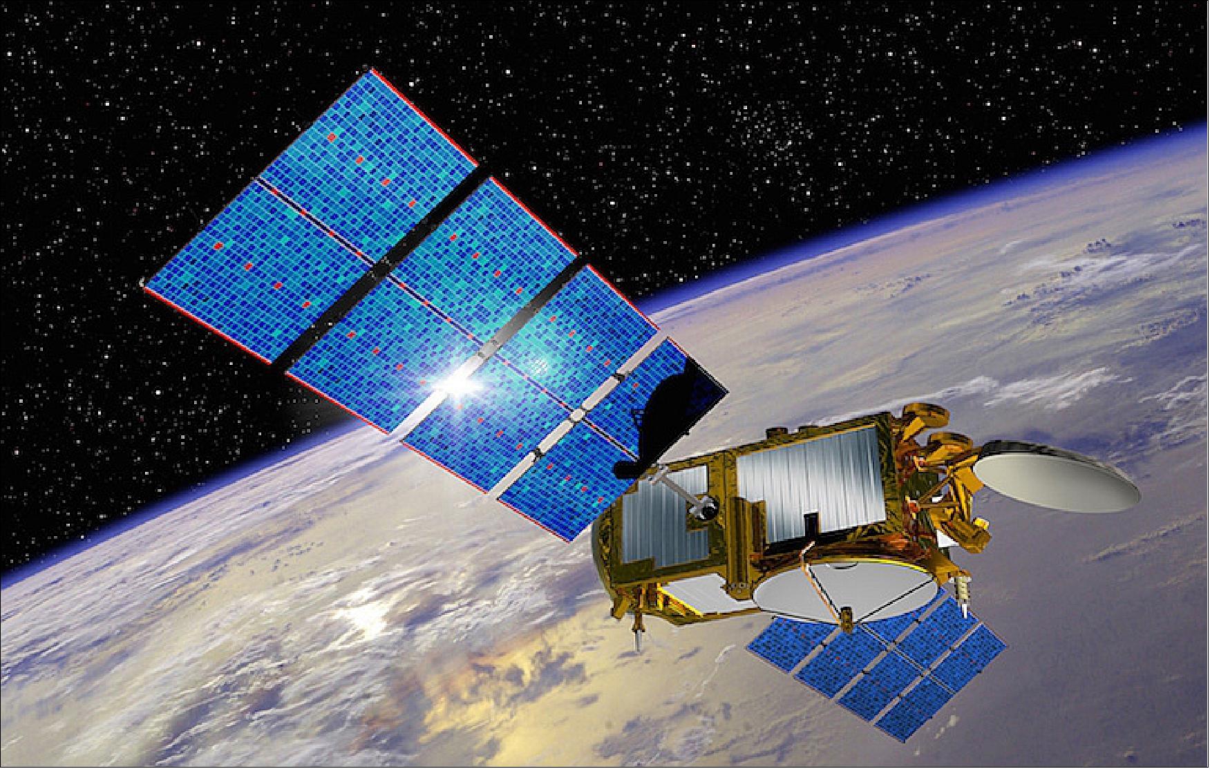
• Like its predecessor Jason-2, the Jason-3 mission employs the Proteus bus of CNES/TAS (Thales Alenia Space) and a payload module, with Thales Alenia Space as the prime contractor of the spacecraft. The CNES contract with TAS followed the early February 2010 approval by the EUMETSAT governments for the required funding of the spacecraft. Jason-3 is three-axis stabilized and nadir pointing - maintained by reaction wheels and magnetic torque rods. 13)
• NOAA will contribute to Jason-3's payload and will also be responsible for the launch of the spacecraft. The payload will consist of the same core instruments as Jason-2: a Poseidon class Ku/C-band radar altimeter to provide the primary ranging measurement, a nadir–looking three frequency (18.7, 23.8, and 34.0 GHz) microwave radiometer (as flown on Jason-2), along with a POD (Precise Orbit Determination) package consisting of a GPS (Global Positioning System) receiver, DORIS (Doppler Orbitography and Radiopositioning Integrated by Satellite), and a LRA (Laser Retroreflector Array), as flown on prior Jason series missions. Two additional instruments (dosimeters from CNES and JAXA) will also be embarked to evaluate the radiation environment. - NOAA has engaged NASA/JPL to act on its behalf to fulfill some of its respective commitments on the flight system development (Ref. 10).
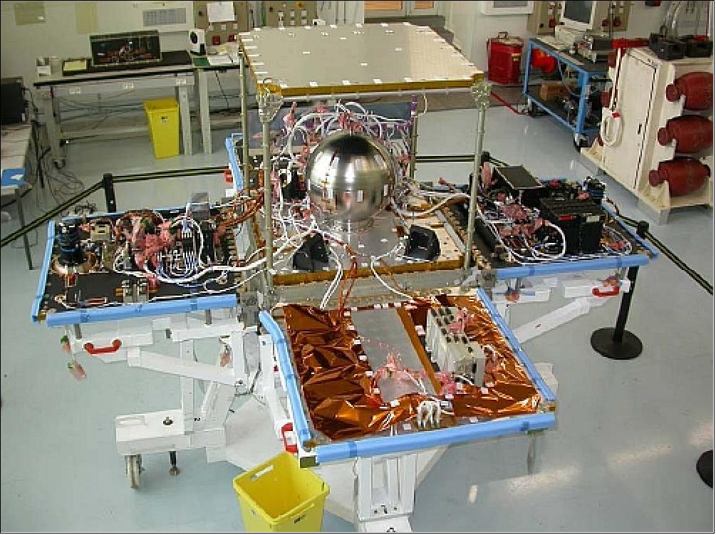
Integration of the Jason-3 platform has been completed in late 2010 and is stored since December 2010.
Like Jason-2, the Jason-3 spacecraft employs the Proteus bus of CNES/Thales Alenia Sapce and a payload module, with Thales Alenia Space as the prime contractor of the spacecraft. Jason-3 is three-axis stabilized and nadir pointing - maintained by reaction wheels and magnetic torque rods. Power (580 W) is provided by two solar panels. A hydrazine propellant system is being used for orbital maintenance. Jason-3 has a launch mass of about 550 kg; the design life is 5 years.
Platform dry mass, payload mass | 277 kg, 255 kg |
Propellant mass | 28 kg of hydrazine |
Spacecraft launch mass | 553 kg |
Electrical power | 550 W (EOL) |
Spacecraft pointing accuracy | 0.15º (1/2 cone) |
Onboard data storage capacity | 2 Gbit |
Spacecraft design life | 5 years |
RF communications: Downlink data rate at 838 kbit/s (S-band, QPSK modulation), uplink at 4 kbit/s (S-band). The CCSDS communication protocol standard is used in the forward and return link mode (use of virtual channels). Convolutional coding is also applied to telemetry.
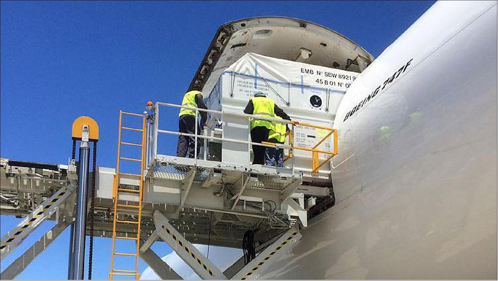
Launch: The Jason-3 spacecraft was launched on January 17, 2016 (18:42.18 UTC) on a SpaceX Falcon 9 v1.1 vehicle from VAFB, CA. 15) 16)
The launch was delayed from July 2015 due to a spacecraft thruster problem. The Jason-3 spacecraft arrived at Vandenberg AFB on June 18, 2015. The launch was delayed following the failed launch of a Falcon-9 vehicle to the ISS (SpaceX CRS-7) on June 28, 2015 from Cape Canaveral, Florida. 17)
In July 2012, NASA contracted SpaceX (Space Exploration Technologies) of Hawthorne, CA to launch Jason-3 aboard a Falcon 9 v1.1 rocket from Complex 4 at VAFB (Vandenberg Air Force Base), CA. 18)
Orbit: Circular non‐sun‐synchronous orbit; 1336 km altitude (2 hour period), inclination = 66.038º, 9.9 day repeat orbits (127 revolutions), ground track repeatability = ±1 km cross‐track at the equator. The drift of the orbital plane with respect to the inertial reference frame is -2º per day.
Mission Status
• December 22, 2020: Though air and sea temperatures worldwide have been quite warm in 2020, the eastern and central Pacific Ocean recently grew milder with the return of La Niña, the cooler sister to El Niño. La Niña brings cool water up from the depths of the eastern tropical Pacific, a pattern that energizes easterly trade winds and pushes warm surface waters back toward Asia and Australia. With this see-sawing of the heat and moisture supply across the Pacific, global atmospheric circulation and jet streams shift. 19)
- During La Niña events, weather patterns typically grow warmer and drier across the southern United States and northern Mexico, noted Josh Willis, a climate scientist and oceanographer at NASA’s Jet Propulsion Laboratory (JPL). Cooler and stormier conditions often set in across the Pacific Northwest of Canada and the U.S. Clouds and rainfall become more sporadic over the central and eastern Pacific Ocean, which can lead to dry conditions in Brazil, Argentina, and other parts of South America. In the western Pacific, rainfall can increase dramatically over Indonesia and Australia. La Niña also can coincide with active Atlantic hurricane seasons, as it did this year.
![Figure 7: The current La Niña event fits into a larger climate pattern that has been going on for nearly two decades. The maps show conditions across the central and eastern Pacific Ocean as observed on November 25, 2020, and analyzed by JPL scientists. The globe on the left depicts sea surface height anomalies measured by the Jason-3 satellite. Shades of blue indicate sea levels that were lower than average; normal sea-level conditions appear white; and reds indicate areas where the ocean stood higher than normal. The expansion and contraction of the surface is a good proxy for ocean temperatures because warmer water expands to fill more volume, while cooler water contracts. The second globe shows sea surface temperature (SST) data from the Multiscale Ultrahigh Resolution Sea Surface Temperature (MUR SST) project. MUR SST blends measurements of sea surface temperatures from multiple NASA, NOAA, and international satellites, as well as ship and buoy observations. (Scientists also use instruments floating within the sea to project underwater temperatures.) [image credit: NASA Earth Observatory image by Joshua Stevens, using data from the Multiscale Ultrahigh Resolution (MUR) project and sea surface height analyses courtesy of Akiko Hayashi/NASA/JPL-Caltech. Story by Michael Carlowicz]](/api/cms/documents/163813/6159066/Jason3_Auto17.jpeg)
- “This 2020 La Niña seems to be peaking,” said Bill Patzert, a retired oceanographer and climatologist from JPL. “It was a bit of a surprise because it evolved quickly and unlike many previous La Niña events it was not preceded by its warm sibling, El Niño.”
- This La Niña fits into a larger climate pattern that has been going on for nearly two decades—a cool (negative) phase of the Pacific Decadal Oscillation (PDO). During most of the 1980s and 1990s, the Pacific was locked in a PDO warm phase, which coincided with several strong El Niño events. But since 1999, a cool phase has dominated.
- “With a few notable exceptions, the PDO has been negative for most of the past 20 years, and that is favorable for La Niña,” said Willis. “Drought patterns across the American Southwest over the past two decades fit with this trend.”
- “The re-emergence of this large-scale PDO pattern tells us there is much more than an isolated La Niña occurring in the Pacific Ocean,” Patzert added. “These shifts can trigger decade or longer droughts in some regions and damaging floods elsewhere.”
- In recent reports issued by the NOAA Climate Prediction Center and the World Meteorological Organization, climatologists forecasted that the current La Niña should last through the 2020-21 northern hemisphere winter. In late November, water temperatures in the central Pacific Ocean were roughly 1.4 degrees Celsius below the long-term average. A La Niña event is declared when average surface water temperatures stay at least 0.5° Celsius below normal in the Niño 3.4 region of the tropical Pacific (from 170° to 120° West longitude) for three months.
- Later in 2021, scientists will have a new tool for observing La Niñas and other trends in global sea level. Following the successful launch of the Sentinel-6 Michael Freilich satellite in November 2020, scientists released some of the first measurements from the new ocean-observing satellite. Engineers and scientists are now calibrating instruments and analyzing data to make sure it correlates properly with long-term records.
- “Christmas came early this year,” noted Willis, who is also NASA’s project scientist for the mission. “And right out of the box, the data look fantastic.”
• On January 17, 2019, Jason-3 celebrates the third anniversary of its launch after having orbited the Earth more than 14,000 times. But it’s not just any anniversary. 20)
- Today, Jason-3 closes its routine operations phase, having accomplished the primary goals defined by its American and European partners – EUMETSAT, the US National Oceanic and Atmospheric Administration (NOAA), the French Space Agency (CNES),NASA/JPL and the European Commission.
- As the satellite and its instruments continue to perform extremely well, from today Jason-3 enters its extended routine operations phase.
- This terminology might not mean much to those outside the meteorological satellite sector, but the importance should not be overlooked. Barring unforeseen circumstances, at least two more years of highly accurate data crucial for climate change monitoring, weather forecasting and safety at sea, and many other applications, can be expected.
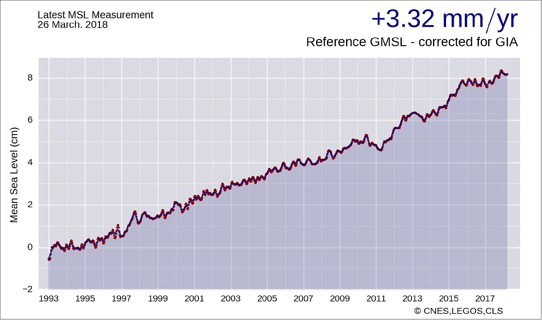
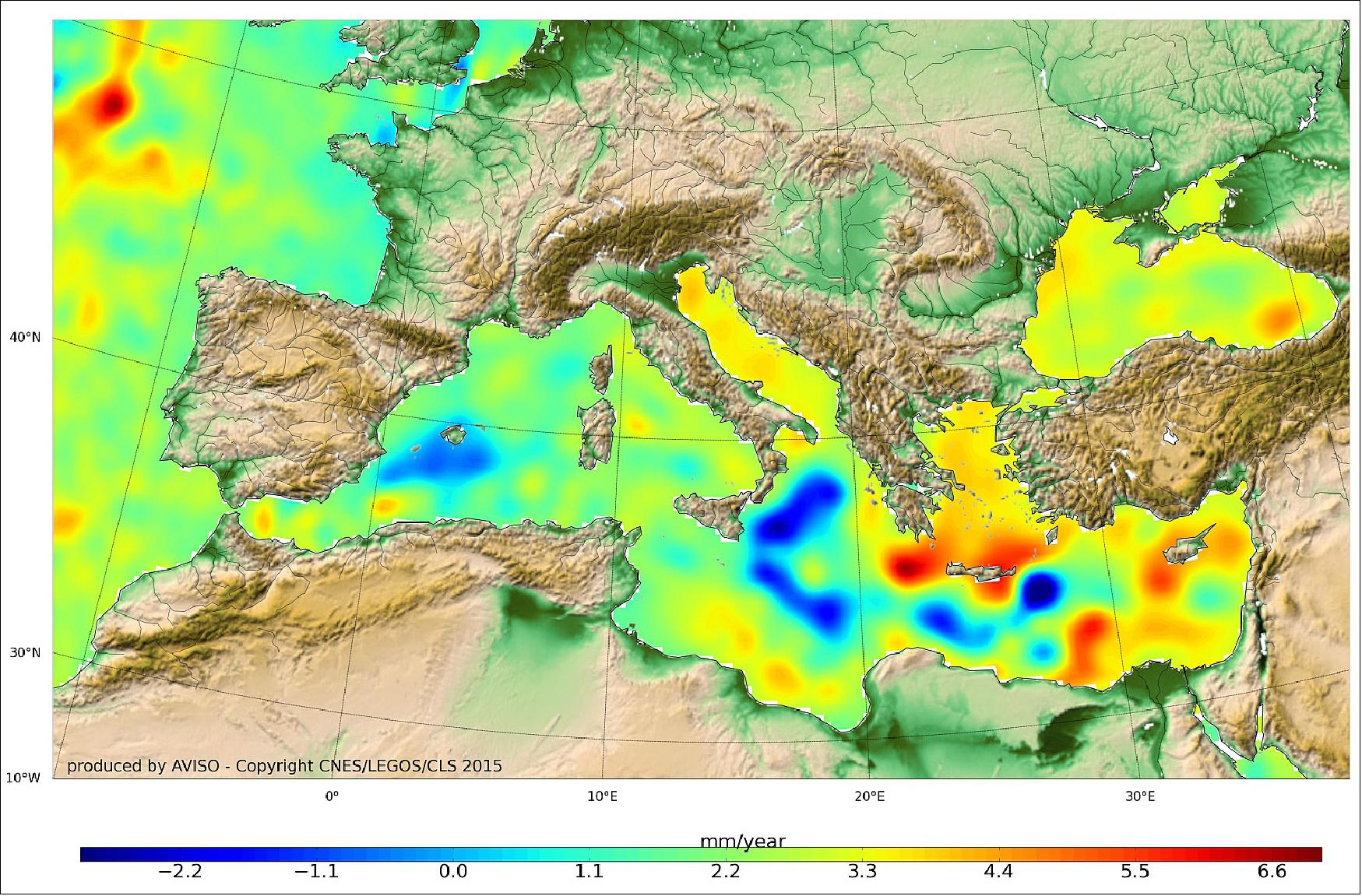
- “Measurements from Jason-3’s altimeter are crucial for climate monitoring,” EUMETSAT Mission Scientist Remko Scharroo said. “Over the past 25 years, the Jason satellites and their predecessors have measured a mean sea level of rise of about 3mm per year. Recently, the first sign that the rise in the mean sea level is accelerating has been observed.
- “Jason-3 is the current High Precision Ocean Altimetry reference mission and is functioning as the reference for other satellite altimeter missions, such as that of Sentinel-3. The marine meteorology community continues to benefit from high-quality wind speed and sea state measurements, which are key factors for improving complex computer modelling needed for weather prediction. And its sea level measurements are inputs for a host of operational ocean applications, such as ocean current monitoring conducted by Europe’s Copernicus Marine Environment Monitoring Service (CMEMS) and hurricane forecasting by NOAA’s National Hurricane Center.”
- Jason-3 is the continuation of an important US/European satellite series that has now been providing vital data on sea level rise and ocean circulation for more than 25 years. This series of satellite radar altimeters measures the peaks and troughs of the sea surface height, or surface topography of the world’s ice-free oceans, every 10 days.
- The data time series began with the 1992 launch of the NASA/CNES TOPEX/Poseidon mission (1992-2006) and was continued by Jason-1 (2001-2013), and by Jason-2, which launched in 2008 and is still in operation. The latter is currently contributing to the generation of a high-resolution map of the mean sea surface.
- “These important missions have provided researchers and society with a rich legacy of unprecedented ocean observations,” NASA/JPL Project Scientist Josh Willis said. “Earth's oceans exert a powerful influence on global climate, and never before have we had such accurate observations of the rate of sea level rise and the change of ocean circulation over time, an important indicator of climate change.”
- Data and images are used for a wide range of scientific, commercial and other applications. Around the globe, operational weather agencies use Jason-3 data for climate forecasting. For many countries, these forecasts are crucial in planning for floods and drought, agricultural strategies and allocating water and energy use.
- With the Jason-3 mission, the quality and precision of the products has kept on improving. As indicated by CNES project scientist Pascal Bonnefond: "Algorithms embedded on the Jason 3 mission were specifically designed to improve data quality in coastal areas, lakes and rivers. These are regions with significant socioeconomic and climatic issues but poorly covered by standard altimetry data in the past."
- The Jason-3 mission is based on solid cooperation between the partners, which capitalizes on the expertise of the different organizations and achieves financial efficiency by sharing costs.
- The Jason-3 Joint Steering Group, with representatives of the mission partners, met in September 2018 and agreed to the extended routine operation phase after the initial three years of the routine operation phase. All parties also expressed their willingness to keep operations going beyond January 2021, should the satellite continue to perform well.
- The long-term future of the high precision ocean altimetry mission is assured through the future Jason-Continuity of Service/Copernicus Sentinel-6 mission. This is a program composed of two successive satellites: Jason-CS A and Jason-CS B, with the first scheduled for launch in November 2020. The Jason-CS program is a successful partnership involving EUMETSAT, ESA, the European Commission, CNES, NOAA, and NASA.
- Jason-3 is expected to play a key role in the commissioning of Jason-CS A, allowing in-flight instrument cross-calibration.
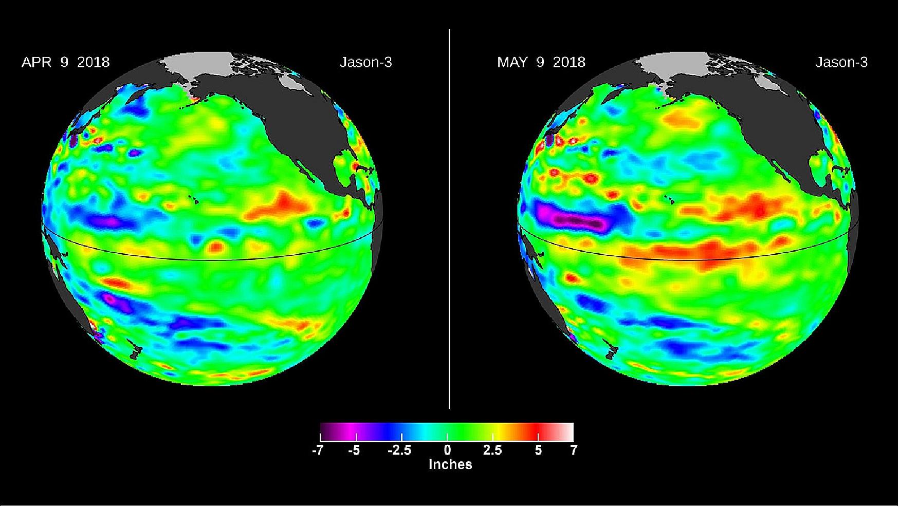
• June 6, 2018: After a mild La Niña late last year, temperatures, convection and rainfall rates in the equatorial Pacific Ocean returned to normal by early April of this year. An April 9 image of sea level height from the U.S./European Jason-3 satellite mission showed most of the ocean at neutral heights. But by the beginning of May, high sea levels began to build up in the Central Pacific (Figure 12). In the tropics, high sea levels are usually caused by a layer of warm water at or below the surface. 21)
- This patch of high sea level is slowly traveling eastward through the tropical Pacific Ocean along the equator. Known as a downwelling Kelvin wave, this type of signal is often a precursor to an El Niño event.
- The Kelvin wave formed after a few short periods when winds changed from the prevailing easterlies to westerly — known as westerly wind bursts — in the far western Pacific in early 2018. In addition, there has been a general weakening of the easterly winds along the equator since January. Both of these wind conditions combine to create the Kelvin wave, which moves east along the equator and results in the spreading of warm water layers that are normally confined to the western Pacific Ocean eastward into the central Pacific. The red pattern visible at the equator on May 9 is the result of this downwelling Kelvin wave.
- During a large El Niño, like the 2015-16 event, a huge area where sea levels are more than a 30 cm higher than normal is visible in Jason-3 images. The high sea level is caused by a thick layer of warm water in the upper several hundred feet of the ocean. Such large El Niño events affect weather and climate across the globe, particularly in the western United States. In California, El Niños usually mean above-average winter rainfall, while Oregon and Washington typically see drier-than-normal winters.
- El Niños happen when a series of Kelvin waves like this one spread warm water from west to east along the equator, causing high sea levels in the Central Pacific and sometimes as far east as the coastlines of Central and South America. The warm water is currently confined to the subsurface, with no warming at the ocean surface — a first indicator of an upcoming El Niño event. But forecasters at agencies like NOAA (the National Oceanic and Atmospheric Administration) and ECMWF (European Centre for Medium-Range Weather Forecasts) will be watching closely for more Kelvin waves like this one as summer approaches.
- NASA's Jet Propulsion Laboratory in Pasadena, California, manages the Jason-3 mission for NASA. NOAA operates Jason-3 in partnership with NASA, the French space agency (CNES), and EUMETSAT (European Organisation for the Exploitation of Meteorological Satellites).
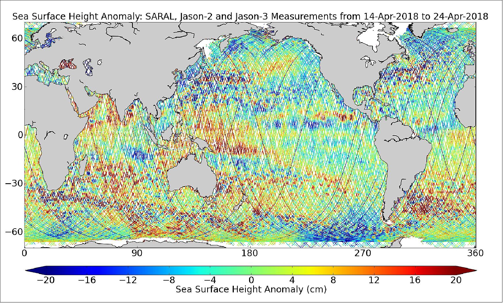
• April 24, 2018: ”Along-Track Near Real-Time SSHA (Sea Surface Height Anomaly) Data.” 22)
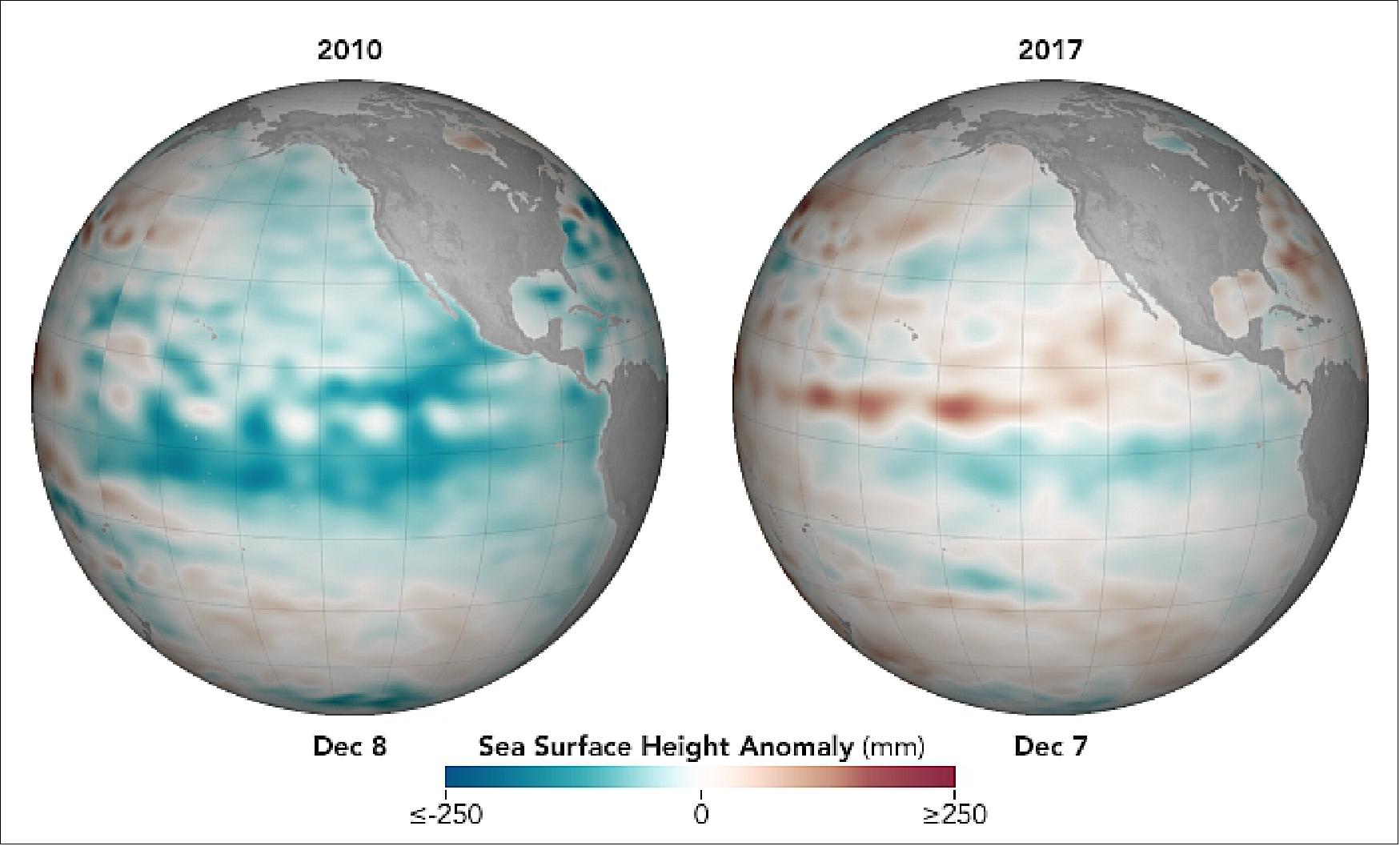
• December 22, 2017: The winter of 2016–17 brought a mild and relatively brief La Niña to the Pacific Ocean, and it now appears that 2017–18 could offer a repeat. On the scale of La Niña events, the conditions developing in the eastern and central Pacific are not yet remarkable, and forecasts suggest they will remain mild. Nonetheless, some familiar atmospheric effects are rippling around the globe. 23)
- La Niña is the cooler sister to El Niño. La Niña draws cool water up from the depths of the eastern Pacific, energizes the easterly winds, and pushes warm surface water back toward Asia. (Note the ripples of warm water moving west across the equator.) In turn, global atmospheric circulation and jet streams shift with the changing heat and moisture supply from the vast Pacific Ocean.
- During La Niña events, the weather tends to grow warmer and drier across the southern portion of North America, from California to Florida. Cooler than normal temperatures usually prevail across western Canada, Alaska, and the U.S. Pacific Northwest. Over the central and eastern Pacific Ocean, clouds and rainfall become more sporadic, while rainfall tends to increase dramatically in Indonesia and the western Pacific. Weather conditions in late 2017 seemed to fit with that pattern.
- After a pattern-defying burst of rain and snow during the La Niña winter of 2016-17, Southern and Central California fell into one of the driest times ever in the region, according to Bill Patzert, a climatologist at NASA’s Jet Propulsion Laboratory. He noted that the region has so far received just 4 percent of normal rainfall since the water (rain) year began on October 1. “Normally, our wettest months are January, February, and March, so there is still a little hope,” Patzert said. “But the La Niña, the notorious ‘diva of drought,’ taking up residence at the equator does not bode well for winter rainfall.”
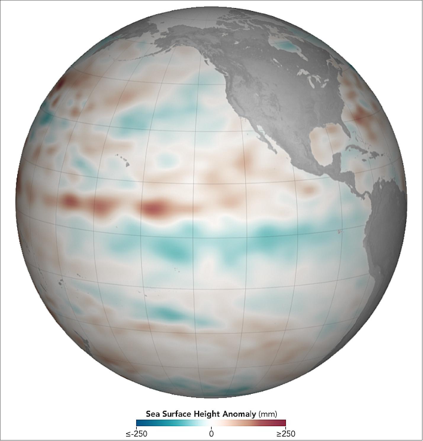
- The measurements were made by altimeters on the Jason-2 and Jason-3 satellites, and show averaged sea surface height anomalies. Shades of red indicate areas where the ocean stood higher than the normal sea level; surface height is a good proxy for temperatures because warmer water expands to fill more volume. Shades of blue show where sea level and temperatures were lower than average (water contraction). Normal sea-level conditions appear in white.
- In reports issued in December 2017 by the NOAA Climate Prediction Center and the World Meteorological Organization, climatologists forecasted that the current La Niña should last through the 2017-18 northern hemisphere winter, before changing to neutral conditions in the late spring of 2018. In early December, water temperatures in the central Pacific Ocean were roughly 1.0 º Celsius below the long-term average. A La Niña event is declared when average surface water temperatures stay at least 0.5° Celsius below normal in the Niño 3.4 region (from 170° to 120° West longitude) for three months. September through November 2017 marked the first such window in the current cycle.
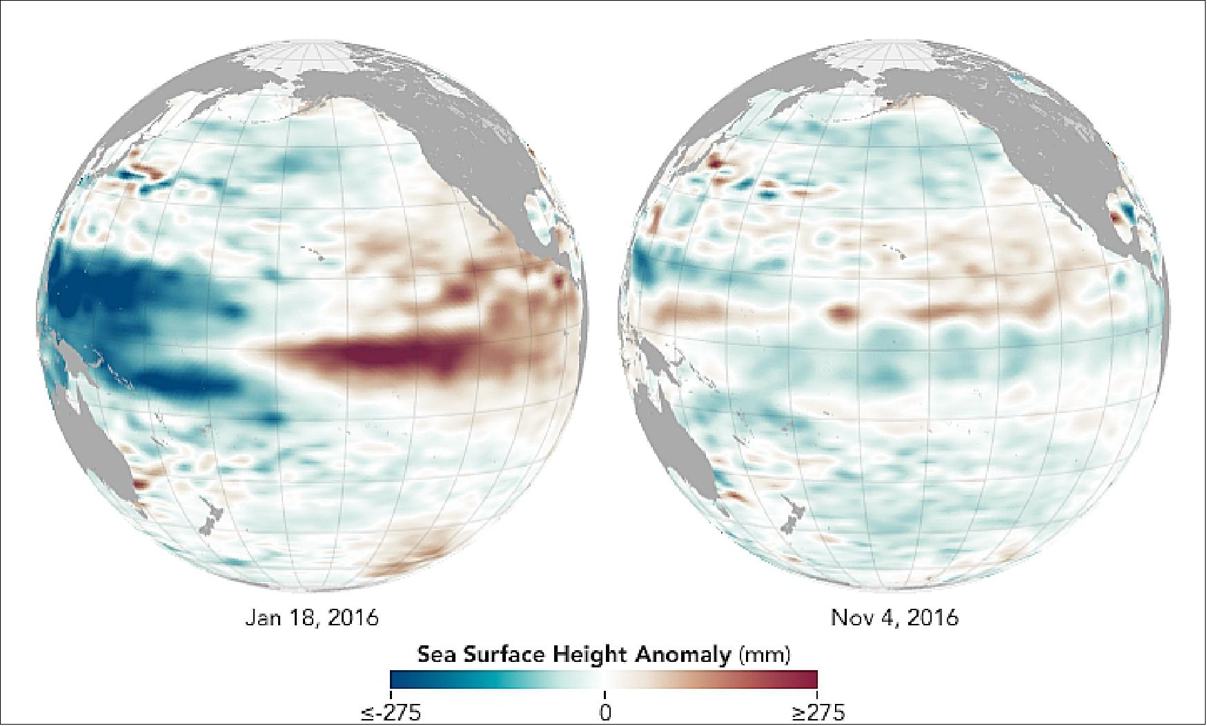
• January 6, 2017: One year ago, the central and eastern parts of the tropical Pacific Ocean were pulsing with heat, a result of one of the most intense El Niño events on record. One year later, La Niña has been relatively quiet, and she does not seem to be staying for long. 24)
- La Niña is the cool sister pattern to El Niño. While El Niño knocks down the easterly trade winds and sloshes warm water from the western Pacific to the Americas, La Niña pulls up cool water from the depths of the eastern Pacific, energizes the easterlies, and pushes the warm water back toward Asia. Regions that often get drenched with rain and snow during El Niño often go dry during La Niña events, and vice versa, as atmospheric circulation and jet streams shift with the changing heat and moisture supply from the vast Pacific Ocean.
- The maps of Figure 16 compare sea surface height anomalies in the Pacific Ocean as observed by NASA scientists on November 4, 2016, near the peak of the current La Niña, and on January 18, 2016, near the peak of last winter’s El Niño. The measurements were made by altimeters on the Jason-2 and Jason-3 satellites, and show averaged sea surface height anomalies. Shades of red indicate areas where the ocean stood higher than the normal sea level; surface height is a good proxy for temperatures because warmer water expands to fill more volume. Shades of blue show where sea level and temperatures were lower than average (water contraction). Normal sea-level conditions appear in white.
- In a report issued in December 2016, the NOAA Climate Prediction Center described the latest La Niña as “weak” and likely changing to neutral conditions in early 2017. La Niña conditions—with surface water temperatures at least 0.5° Celsius below normal in the central and eastern Pacific (the Niño 3.4 region from 170° to 120° West longitude) — began to surface in July and August 2016. During last year’s El Niño, surface water temperatures were as much as 2.5°C above the 1981-2010 norm. During the current La Niña, temperatures have not dropped more than 1 degree below normal.
- “Last year’s Niño was huge in area, duration, and magnitude,” said Bill Patzert, a climatologist at NASA’s Jet Propulsion Laboratory. “My take is that because it lasted so long and covered such a large area, it damped the return of strong trade winds needed for a healthy Niña. Note the strong positive heat content north of the equator—the entire tropical Pacific between Central America and Hawaii—that lingered into the fall.”
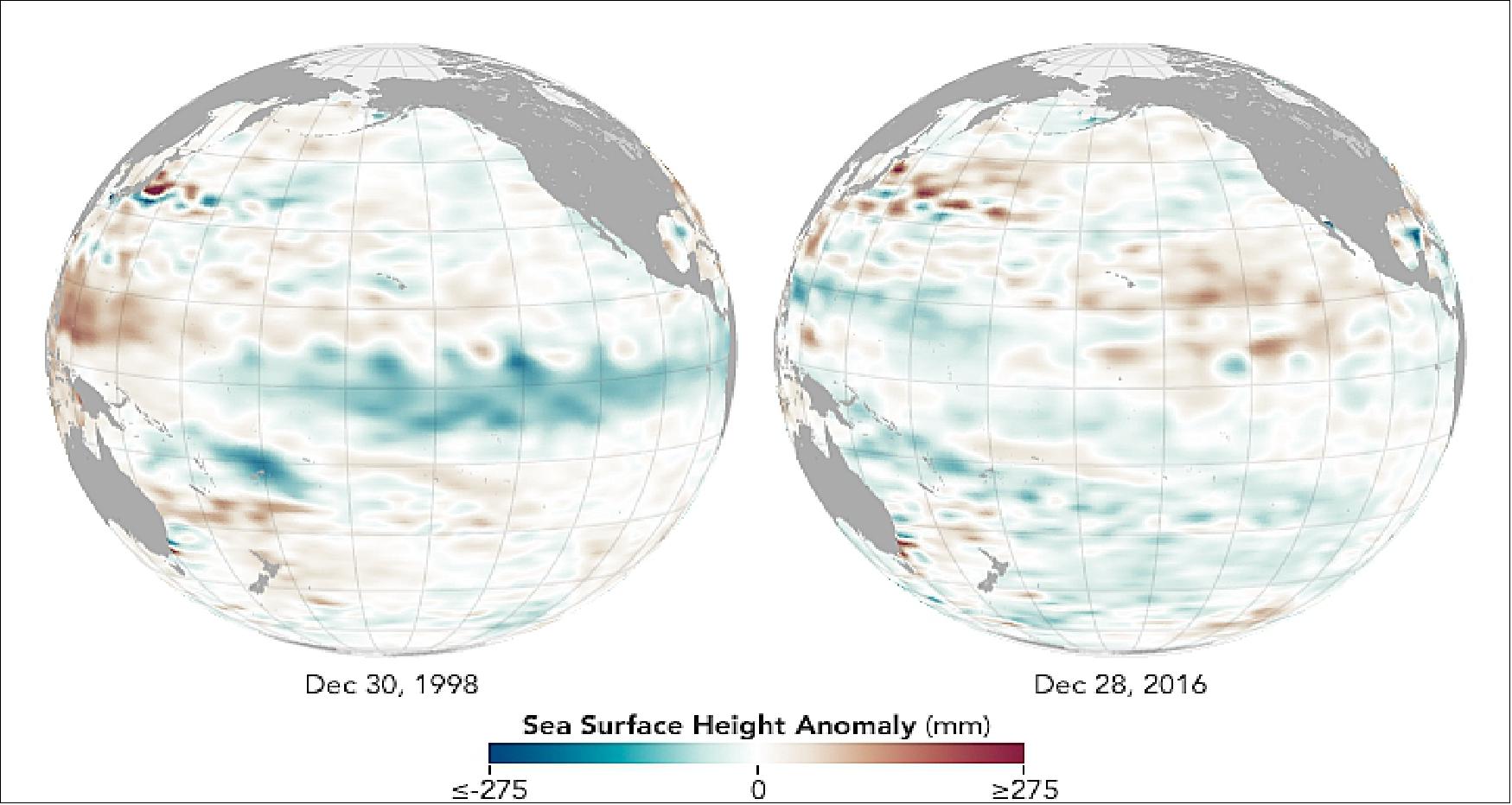
- The patterns following the great El Niño of 2015–16 have been starkly different from what occurred after the last major event. In 1997-98, very warm El Niño conditions persisted for roughly 13 months, but were then followed by roughly 32 months of well-below-normal (La Niña) water temperatures in the eastern Pacific (Figure 17). In 2015–2016, water temperatures and sea surface heights were above normal for 19 months, first weakly and then with great gusto in late 2015. But this event has been followed by just five months of weak La Niña conditions that are already fading.
- “As with investing, past performance does not guarantee future results for the ENSO cycle,” wrote ocean climatologist Mike McPhaden of the NOAA Pacific Marine Environmental Laboratory in an email. “Though there are common features that characterize all El Niños and La Niñas, each one is different with its own unique personality. That a strong La Niña followed a strong El Niño in 1997-98 does not mean that all strong El Niños are followed by strong La Niñas.”
- “What factors have limited the growth of this La Niña event is a great research question, one that I am sure many people will be investigating in the near future,” McPhaden added. “The climate system is very complex, and many processes are at work at any given point in time and space. It could be just the randomness of the climate system that kept this La Nina from taking full flight. Or maybe it is the fact that the Pacific Decadal Oscillation has been in a mostly warm state since 2014, with elevated temperatures in the tropical Pacific making it harder to develop cold anomalies there.”
- Mike Halpert, deputy director of the NOAA Climate Prediction Center, noted that the current pattern is somewhat similar to 1982–83, when another strong El Niño was followed by a relatively modest La Niña. “Just when you think you have seen everything and think you know what to expect, something happens that you just can’t explain,” he noted. “There are many rhythms and natural variabilities, and nature will always keep it interesting.”
• November 24, 2016: With the decision to release the GDR (Geophysical Data Record), the Jason-3 partner agencies CNES, NOAA, NASA/JPL and EUMETSAT ensure the availability of the full suite of Jason-3 products and confirm Jason-3 as the operational reference mission for ocean altimetry. This also enlarges the portfolio of ocean products offered by the Copernicus Program of the European Commission. 25)
- The GDR, available within 60 days, is the most accurate and complete among the Jason-3 products. It offers fully validated sea surface height data for the international science community. In the context of operational oceanography, for example, it is used primarily for ocean reanalysis.
- The product also delivers data for climate monitoring, here in particular climate model verification, sea level monitoring and climate change assessment. The IPCC (International Panel for Climate Change) relies on the GDR for its reports.
- The NRT (Near-Real-Time) OGDR ( Operational Physical Data Records) products, disseminated to the EUMETSAT Users via EUMETCast and the GTS (Global Telecommunications System), and the IGDR (Interim Geophysical Data Records), distributed by CNES, have been available since 1 July.
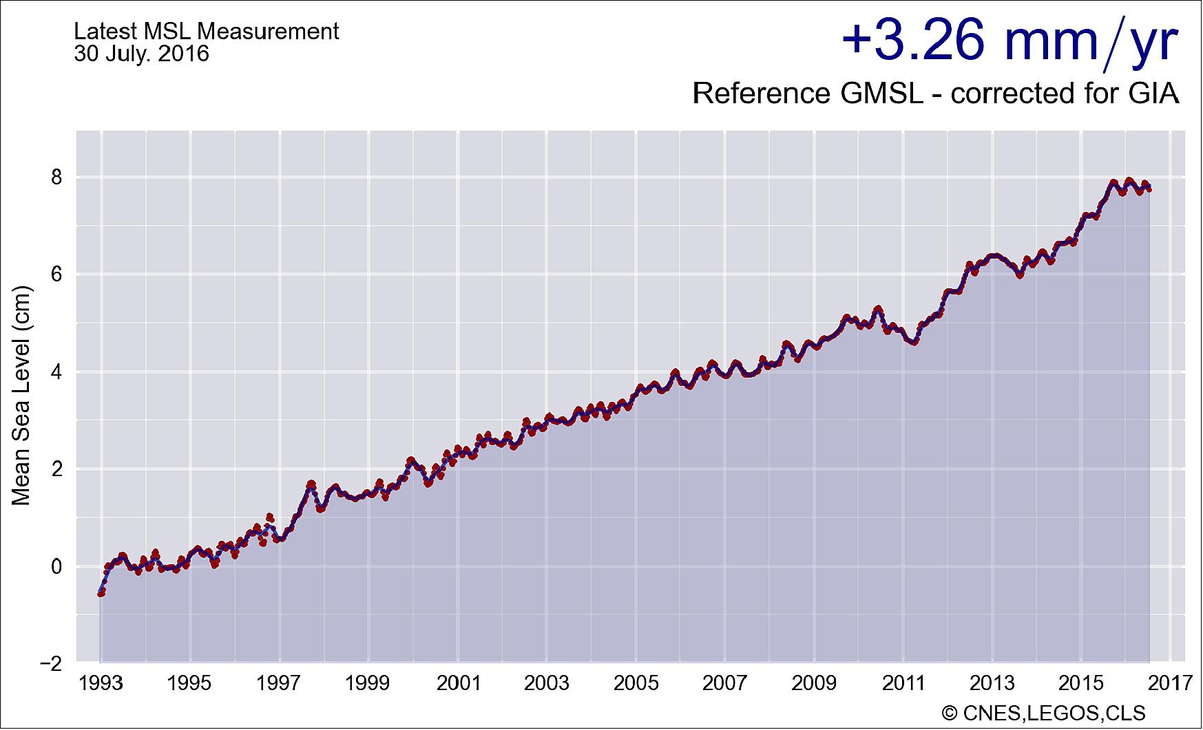
Legend to Figure 18: MSL (Mean Sea Level), GMSL (Global Mean Sea Level), GIA (Glacial Isostatic Adjustment).
• On July 1, 2016, an important milestone has been reached in the commissioning of the US-European Jason-3 ocean-monitoring mission with the release of the OGDRs (Operational Geophysical Data Records) in NRT (Near-Real Time), and the NTC (Non-Time Critical) IGDR (Interim Geophysical Data Record) to all users. 26)
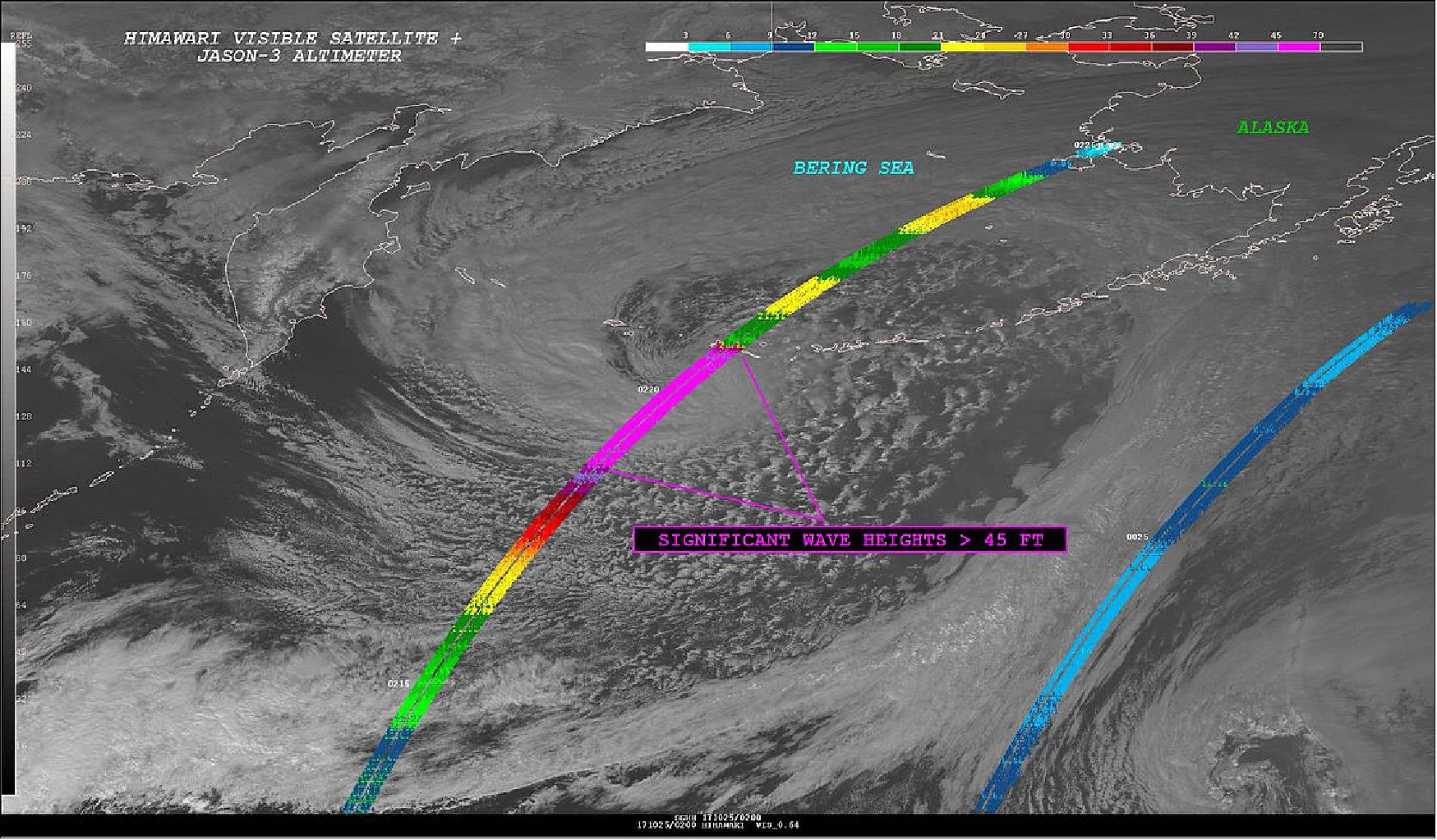
- The OGDRs include estimates of significant wave height, wind speed, and a first estimate of sea surface height based on orbit data and atmospheric corrections available in real time. They are disseminated to users within three hours of observation. IGDRs are distributed within two days of observation and provide more accurate estimates of sea surface height thanks to improved orbit determination.
- Over recent months, engineers from CNES, EUMETSAT, NOAA and NASA and scientists from the international Ocean Surface Topography Science Team have been evaluating the Jason-3 OGDRs and IGDRs. During this period, Jason-3 was flying in tandem with Jason-2, approximately 80 seconds apart, for the purpose of cross-calibration of sea surface height measurements at sub-centimeter level.
- The OGDR and IGDR products will now be used worldwide for sea state forecasting, monitoring of marine environment and assimilation into models of the ocean or the coupled ocean-atmosphere system for ocean and seasonal forecasting.
- Saleh Abdalla, a scientist at ECMWF, said: “The assimilation of Jason-3 OGDR sea surface height and significant wave height into the ECMWF Integrated Forecasting System improves the operational medium- to long-range weather forecasts and surface wind speed and total column water vapor measurements are important for model verification."
- During the first Jason-3 verification workshop on 21 June, the European and US partners in the program also decided to switch the operational service from Jason-2 to Jason-3 and to move Jason-2 to an interleaved orbit in Mid-September, to increase space and time coverage in line with user needs.
- EUMETSAT Director of Operations and Services to Users Livio Mastroddi said: “This milestone opens EUMETSAT’s delivery of operational Jason-3 data services to the EU Copernicus flagship Earth observation program.”
• March 16, 2016: Jason-3, a new U.S.-European oceanography satellite mission with NASA participation, has produced its first complete science map of global sea surface height, capturing the current signal of the 2015-16 El Niño. 27)
- Over the past several weeks, mission controllers have activated and checked out Jason-3’s systems, instruments and ground segment, all of which are functioning properly. They also maneuvered Jason-3 into its operational orbit, where it now flies in formation with Jason-2 in the same orbit, approximately 80 seconds apart. The two satellites will make nearly simultaneous measurements over the mission’s six-month checkout phase to allow scientists to precisely calibrate Jason-3’s instruments.
- John Lillibridge, NOAA Jason-3 project scientist in College Park, Maryland, said comparisons of data from the two satellites show very close agreement. “It’s really fantastic. The excellent agreement we already see with Jason-2 shows us that Jason-3 is working extremely well, right out of the box. This kind of success is only possible because of the collaboration that’s been developed between our four international agencies over the past quarter century.”
- Once Jason-3 is fully calibrated and validated, it will begin full science operations, precisely measuring the height of 95 percent of the world’s ice-free ocean every 10 days and providing oceanographic products to users around the world. Jason-2 will then be moved into a new orbit, with ground tracks that lie halfway between those of Jason-3. This move will double coverage of the global ocean and improve data resolution for both missions. This interleaved mission will improve our understanding of ocean currents and eddies and provide better information for forecasting them throughout the global oceans.
- NASA and CNES shared responsibilities for Jason-3’s satellite development and launch. CNES provided the Jason-3 spacecraft, while NASA was responsible for management of launch services and countdown operations for the SpaceX Falcon 9 rocket. NASA and CNES jointly provided the primary payload instruments. CNES and NOAA are responsible for satellite operations, with instrument operations support from JPL, which is managing the mission for NASA. Upon completion of Jason-3’s commissioning phase, CNES will hand over satellite mission operations and control to NOAA. Processing, archival and distribution of data products to users worldwide is being carried out by CNES, EUMETSAT and NOAA.
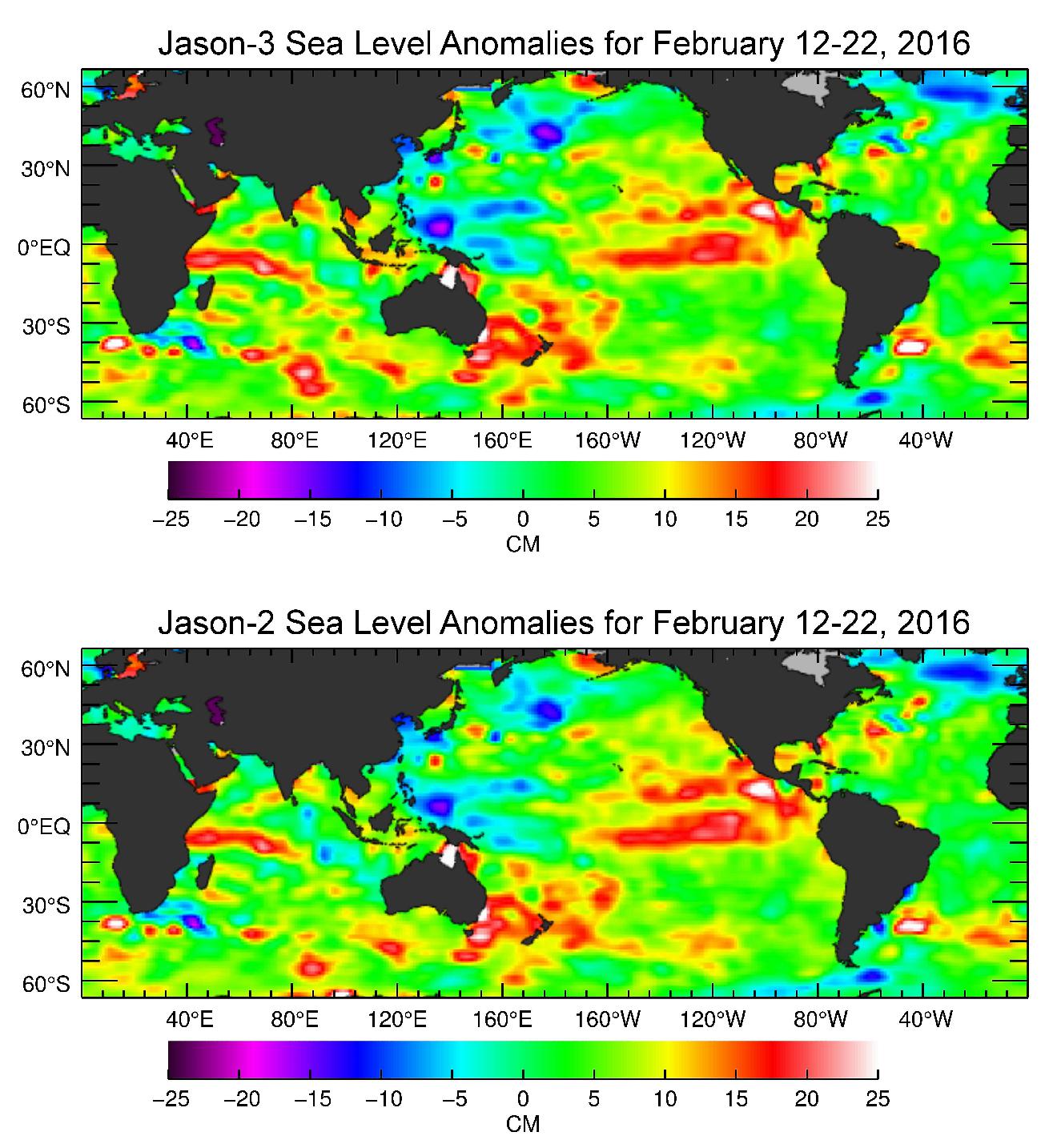
Legend to Figure 19: The map was generated from the first 10 days of data collected once Jason-3 reached its operational orbit of 1,336 km in Feb. 2016. It shows the state of the ongoing El Niño event that began early last year. After peaking in January, the high sea levels in the eastern Pacific are now beginning to shrink.
Date | Milestone | Description |
Jan. 17, 2016 | Jason-3 launch | The Jason-3 spacecraft was launched aboard a SpaceX Falcon 9 rocket on January 17, 2016. |
Jan. 18, 2016 | Jason-3 LEOP (Launch and Early Orbit Phase) | The spacecraft and instrument teams have completed the 3-day LEOP with the successful activation of the spacecraft sub-systems and all the science instruments. |
Feb. 12, 2016 | Jason-3 to reach final orbit | Jason-3 entered its final orbit, directly behind Jason-2. The satellites are flying 560 km apart with only 1 minute and 20 seconds between them. Shortly after reaching this milestone, NESDIS will release first Jason-3 demonstration products to the NWS Ocean Prediction Center and National Hurricane Center for early evaluation. |
May 24, 2016 | Official satellite handover from CNES to NOAA | A handover review for satellite operations will be conducted between CNES and NOAA in Suitland, MD. |
June 21, 2016 | First Verification Workshop to approve official release of operational products | Workshop to announce official release of significant wave height, ocean current, and sea surface heights as Jason 3 operational products. |
Sept. 1, 2016 | Begin Jason-2’s move to interleave orbit | Jason-2 will begin its move to an interleave orbit, leaving Jason-3 to operate in its final orbit alone. |
Dec. 15, 2016 | Final Verification Workshop | Workshop to announce the official release of the Jason-3 climate data records for use by the climate community. |
• Feb. 11,2016: The newly launched Jason-3 satellite should move into its final orbit within days, trailing its counterpart, Jason 2, by only two minutes. The two spacecraft, some 1,336 km above Earth, will measure sea levels in virtually the same ocean conditions as they fly in formation. 29)
- For the first six months, the measurements mainly will be used to calibrate Jason-3’s instruments by comparison to Jason-2, aloft since 2008. After Jason-3’s checkout phase, full science operations begin.
• January 21, 2016: Four days after its launch on 17 January, the Jason-3 high-precision ocean altimetry satellite is delivering its first sea surface height measurement data in near-real time for evaluation by engineers from CNES, EUMETSAT, NASA and NOAA and scientists from the international Ocean Surface Topography Science Team. 30)
- The data started to be acquired, processed in realtime at CNES and products started to be delivered shortly after the successful completion of the LEOP ( Launch and Early Orbit Phase) carried out by CNES. This performance is owed to the experience gained through the sustained partnership between CNES, EUMETSAT, NASA and NOAA.
- To ensure consistency of the measurements and climate data records from the Jason orbit, Jason-3 will be cross-calibrated with Jason-2 before routine operations. As of the beginning of February, the two satellites will therefore be flying in a tandem configuration, one minute apart of each other.
• After launch, control of the spacecraft was taken over by CNES, which over the next three days will perform early orbit phase operations such as configuration of the platform and the payload. 31)
• Jason-3 entered orbit about 25 km below Jason-2. The new spacecraft will gradually raise itself into the same 1,336 km orbit and position itself to follow Jason-2's ground track, orbiting about a couple of minutes behind Jason-2. The two spacecraft will fly in formation, making nearly simultaneous measurements for about six months to allow scientists to precisely calibrate Jason-3's instruments (Ref. 15).
• SpaceX’s own secondary objective of soft landing the Falcon 9 first stage, was partially successful. Although the booster was targeted precisely to an oceangoing barge in the Pacific Ocean, it ultimately crash landed when one of the four landing legs apparently failed to deploy fully causing the rocket to tip and fall on the deck. 32)
Sensor Complement
In addition to the sensor complement, 2 experiments will be embarked on Jason-3: Carmen-3 and LPT for radiation effects with the same constraints as for Jason-2 (Ref. 11).
Drift requirements : Specific Seattle OSTST (Ocean Surface Topography Science Team) recommendation: 33)
• J3-TARG-PROD-147: As a goal, Jason-3 shall measure globally averaged sea level relative to levels established during the cal/val phase with zero bias ±1 mm (standard error) averaged over any one year period.
• J3-TARG-SYST-335: In order to satisfy the stability goal of reaching an uncertainty of less than 1mm/year in mean sea level change, allocations shall be given and enforced to the different components of the JASON-3 system that contribute to this measurement.
• J3-GUID-SYST-336. Tentative allocation for mean sea level change error budget is as follows:
- External geophysical correction: 0.1 mm/yr
- Orbit drift: 0.1 mm/yr
- Microwave radiometer wet troposphere correction: 0.7 mm/yr
- Sigma naught (σο) drift impact on sea state bias through wind speed): 0.1 mm/yr.
| OGDR (Operational Geophysical Data Record) | IGDR (Interim Geophysical Data Record) | GDR (Geophysical Data Record) | GOALS |
Altimeter range (RMS) | 4.5 cm | 3 cm | 3 cm | 2.25 cm |
RMS orbit (radial) | 5 cm (a) | 2.5 cm | 1.5 cm | 1 cm |
Total RSS sea surface height | 6.8 cm | 3.9 cm | 3.4 cm | 2.5 cm |
Significant wave height | 10% or 0.5 m (b) | 10% or 0.4 m (b) | 10% or 0.4 m (b) | 5% or 0.25 m (b) |
Wind speed | 1..6 m/s | 1.5 m/s | 1.5 m/s | 1.5 m/s |
Sigma naught | 0.7 dB | 0.7 dB | 0.7 dB | 0.5 dB |
System drift |
|
|
| 1 mm/year (c) |
Legend to Table 3: (changes compared to Jason-2 are in blue)
(a) Real time DORIS onboard ephemeris
(b) Whichever is greater
(c) Jason-3 shall measure the globally averaged sea level relative to the levels established during the cal/val phase with zero bias ±1 mm (standard error) averaged over any one year period.
Operational Service Specifications : Reference TP4-J0-STB-32-CNES v 1.0
• Data Products requirements : Level2 ocean type products (geolocated and along-track geophysical products)
• NRT (Near-Real Time) products : Operational Geophysical Data Record (OGDR) : produced in near real time (3-5 hours)
- Fast Quality Control & Check : Elementary and automatic controls, product delivered in any case
- Priority given data latency with respect to validation and auxiliary data availability + forecast meteo files used.
• OFL (Off-Line) products : Interim Geophysical Data Record (IGDR) : produced in 1.5 days
- Quality Control & Check : Product not delivered in case of problems detected; Products validated by SALP/Calval activities (Calval chain + verification step); Possible reprocessing in case of quality problems.
- Improvement of : orbit quality (MOE), pole location data, restituted DORIS USO frequency, altimeter/radiometer calibrations, analyzed meteorological fields, dynamic atmospheric corrections applied.
• Geophysical Data Record (GDR) : produced in 60 days
- Quality Control & Check : Products fully validated by experts (CNES and JPL); Possible reprocessing
- Improvement of: orbit quality (POE), more accurate pole location data, more accurate dynamic
atmospheric corrections.
Product | OGDR | IGDR | GDR |
Processed by | NOAA and EUMETSAT | CNES | CNES |
Disseminated by (systematic, electronic) | NOAA and EUMETSAT | NOAA and CNES | NOAA and CNES |
Latency | 3-5 hours | 1.5 days | ~60 days |
1 Hz | OGDR-SSHA | IGDR-SSHA | GDR-SSHA |
1 Hz | OGDR | IGDR | GDR |
Waveforms | - | S-IGDR | S-GDR |
Structure | segment | pass | pass |
| segment | day | cycle |
System : AMR on-board cold space calibration • Lisbon OSTST recommendation, San Diego OSTST decision • Satellite pitch maneuvers (80°off nadir). Satellite: • Slight modification of satellite OBSW (Tx OFF for safety improvement, PIM structure panels) • Change in PIM structure panels for compliance with each potential launch vehicle by waiting for the selection. Poseidon-3B Altimeter: • Implementation of a single mode with on-board automatic transitions between DIODE/DEM tracking and autonomous tracking, with respect to the satellite position • Poseidon-3B DEM upload is now possible without mission interruption. DORIS: • New generation DGXX-S taking into account lessons learned from Jason-2 • Change of DORIS antenna location for compliance with each potential launch vehicle while waiting for the selection • Improvement in modeling the Solar Panels position. AMR (Radiometer): • Mostly recurring design with improvement of the instrument thermal control and stability (lesson learned from Jason-2 experience). GPSP: • Different receiver but with same basic design as on JASON-1/2 • Not mission critical but applying further updates for radiations hardened parts and shielding. Launcher: • Launch vehicle : Falcon 9 (SpaceX) • New Payload Processing Facility (PPF) at Vandenberg : SpaceX PPF Ground: Capability to operate simultaneously JASON-2 and JASON-3 • Addition of stations for the “formation flight” phase : Barrow (NOAA) and Usingen2 (EUM) • JASON-2 and JASON-3 operations “merging” considered after the launch Product Processing : • Development of a “digital retracking” to be used for Jason-3 GDR allowing to take into account the actual instrument features before launch and in-orbit and to better estimate the low sea states. |
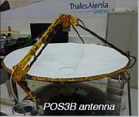
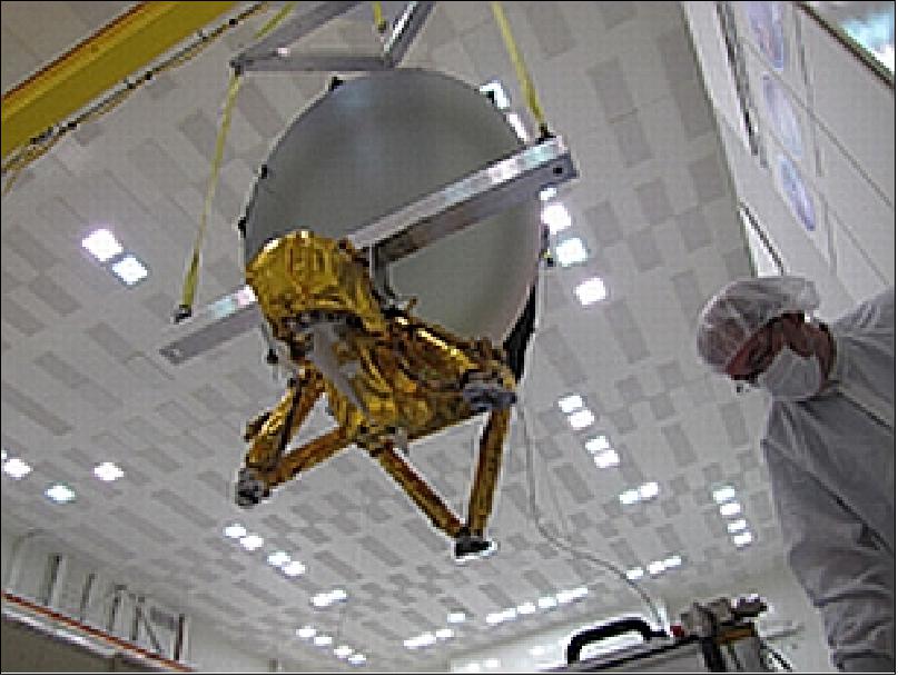
Poseidon-3B Altimeter
Poseidon-3B is funded by EUMETSAT and of Poseidon-2 heritage (built by Thales Alenia Space). The Poseidon-3B dual-frequency (5.3 and 13.6 GHz) nadir-looking radar altimeter continues to be the key instrument in this spaceborne observation program. The objective is to map the topography of the sea surface for calculating ocean surface current velocity and to measure ocean wave height and wind speed. Poseidon-3 has a measurement precision identical to its predecessor Poseidon-2.
Transmission frequencies | 5.3 GHz (C-band), 13.575 GHz (Ku-band) |
Transmitted pulse width | 105.6 µs |
Bandwidth | 320 MHz (Ku-band and C-band) |
PRF (Puls Repetition Frequency) | 2060 Hz interlaced (3 Ku-1C- 3 Ku-band) |
Peak output power | 8 W for Ku-band, 25 W for C-band |
Max. RF power output to antenna | 38.4 dBm Ku-band, 42 dBm for C-band |
Antenna diameter | 120 cm |
Antenna beamwidth | 1.28º (Ku-band), 3.4º (C-band) |
Noise figure | 3.2 dB (Ku-band), 0.9 dB (C-band) |
Data rate | 22.5 kbit/s including waveform data and onboard parameters |
Redundancy | Yes |
Special features | Solid-State Power Amplifier (SSPA). |
Scanning technique | Nadir-only viewing, sampling at 30 km intervals along track |
Instrument mass, power | 70 kg, 78 W |
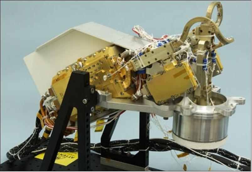
In addition, Poseidon-3B features an experimental mode to support measurements closer to coastal zones, as well as on lakes and rivers. This will be achieved by an open loop tracker: the satellite to surface distance will be estimated by the altimeter using the real-time orbit position predicted by DIODE (on board navigator based on DORIS receiver) and using the elevation of the surface with respect to the Earth GRIM5 geoid stored in a DEM (Digital Elevation Model) within the altimeter. The instrument's RFU is recurrent from Poseidon-2, while the PCU (Processing & Control Unit) largely reuses electronics from the SIRAL radar altimeter on the CryoSat mission of ESA (European Space Agency).
AMR-2 (Advanced Microwave Radiometer-2)
The AMR-2 instrument is funded by NOAA and provided by NASA/JPL with the objective to measure the altimeter signal path delay due to tropospheric water vapor. 35)
AMR-2 is a passive microwave radiometer measuring the brightness temperatures in the nadir column at 18.7, 23.8, and 34 GHz, providing path delay correction for the altimeter (the brightness temperatures are converted to path-delay information). The 23.8 GHz channel is the primary water vapor sensor, the 34 GHz channel provides a correction for non-raining clouds, and the 18.7 GHz channel provides the correction for effects of wind-induced enhancements in the sea surface background emission. 36)
The AMR-2 consists of two subsystems: ESA (Electronics Structure Assembly) and RSA (Reflector Structure Assembly). The ESA is developed by JPL, while the RSA is developed by ATK Space Systems, San Diego, CA.
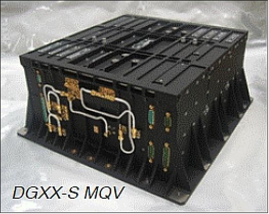
DORIS (Precise Orbit Determination System)
The Doris system uses a ground network of 60 orbitography beacons around the globe, which send signals at two frequencies to a receiver on the satellite. The relative motion of the satellite generates a shift in the signal's frequency (called the Doppler shift) that is measured to derive the satellite's velocity. These data are then assimilated in orbit determination models to keep permanent track of the satellite's precise position (to within three centimeters) on its orbit.
This instrument is funded by EUMETSAT and supplied by CNES with a new generation (DGXX-S) taking into account lessons learned from Jason-2. Improvement in modeling solar panels position will be made. Current model improvements will be integrated: albedo and infrared pressure, ITRF 2008, pole prediction, Hill along-track empirical acceleration, on-board USO frequency prediction, ... allowing a more and more accurate Diode navigation tool. 38)
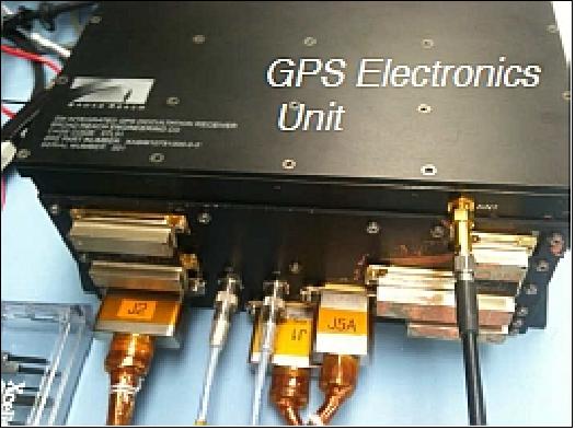
GPSP (GPS Payload)
The GPSP uses the Global Positioning System (GPS) to determine the satellite's position by triangulation, in the same way that GPS fixes are obtained on Earth. At least three GPS satellites determine the mobile's exact position at a given instant. Positional data are then integrated into an orbit determination model to track the satellite's trajectory continuously.
The GPSP instrument is funded by NOAA and supplied by NASA, it will be a different receiver but with same basic (blackjack) design as on Jason-1 and 2. No changes to data processing or products with expect same or better performance as on Jason-2.
LRA (Laser Retro-reflector Array)
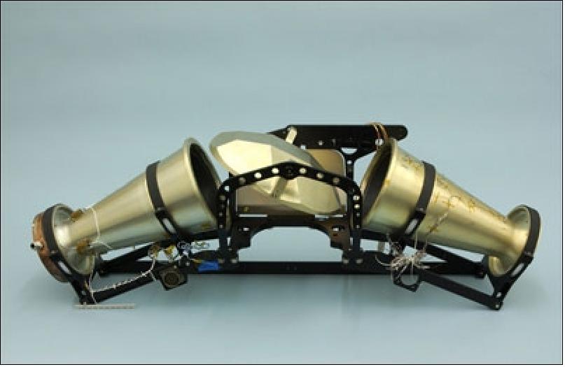
LRA is a JPL instrument of TOPEX/Poseidon heritage, built by ITE Inc. under NASA/GSFC contract - funded by NOAA. LRA provides a reference target for satellite laser ranging (SLR) measurements, which are necessary to calibrate the POD system and the altimeter throughout the mission. The LRA is placed on the nadir face of the satellite. It is a totally passive unit that consists of nine quartz corner cubes arrayed as a truncated cone with one in the center and the other eight distributed azimuthally around the cone. This arrangement allows laser ranging at FOV (Field-of-View) angles of 360º in azimuth and 60º elevation around the perpendicular. The retroreflectors are optimized for a wavelength of 532 nm (green), offering a FOV of about 120º. The LRA instrument mass is 2.2 kg.
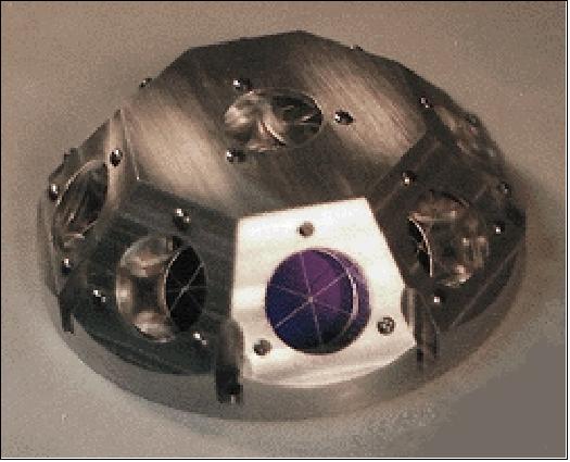
The LRA is a passive instrument that acts as a reference target for laser tracking measurements performed by ground stations. Laser tracking data are analyzed to calculate the satellite's altitude to within a few millimeters. However, the small number of ground stations and the sensitivity of laser beams to weather conditions make it impossible to track the satellite continuously. That is why other onboard location systems are needed.
Passenger Instruments
JRE (Joint Radiation Experiment) - CARMEN-3 + LPT
CARMEN (CARacterization and Modeling of ENvironment) is an instrument concept dedicated to space environment measurement: orbital debris, high and low energy particles. CARMEN-3 is composed of the ICARE-NG module and an additional sensor AMBRE. ICARE-NG is a dedicated instrument to study the influence of space radiation and their effects on electronic components. AMBRE is a type of sensor which is able to detect low level ions and electrons.
CARMEN-3 instrument has particular mission objectives as well as objectives related to the satellite:
• Scientific objectives for ICARE-NG: to allow the measurement of charged particles fluxes and the effects of these particles fluxes on under test electronic components.
• Scientific objectives for AMBRE: to allow the measurement of low energy charged particles fluxes responsible for electrostatic discharges.
• Mission objectives for CARMEN-3 associated with JASON-3: to allow the local radiative environment characterization and the evaluation of the potential drifts of the equipments in particular due to radiation from South Atlantic Anomaly (SAA), and to participate in the data cross calibration with the LPT instrument in the frame of JRE (Joint Radiation Experiment).
Carmen-3 (CNES instrument) is a dosimeter used to improve knowledge of particularly aggressive radiation in Jason's orbit.
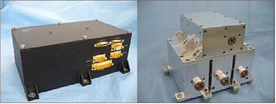
LPT (Light Particle Telescope)
LPT is a detection unit of JAXA (Japan Aerospace Exploration Agency), Tokyo, Japan. LPT complements the radiation measurements of Carmen-2. In June 2006, JAXA and CNES signed a MOU (Memorandum of Understanding) with the intent to load the JAXA instrument LPT (Light Particle Telescope) onto the Jason-2 spacecraft of CNES. 39)
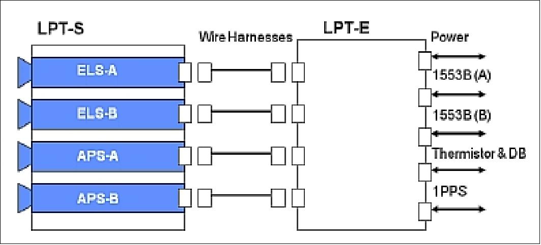
LPT consists of two units, which are LPT-E and LPT-S. Figure 29 shows the external views of LPT-E (left) and LPT-S (right). A block diagram of LPT is shown in Figure 30. LPT-E is mounted inside of the satellite and LPT-S is outside.
LPT-E provides functions of the electrical I/F with the Jason-2 satellite system. It receives primary power supply from satellite system and provides sensors and electrical circuits with secondary power. It also receives telecommands and sends telemetry data via the MIL-1553B bus using protocols specified by the PROTEUS standard satellite bus which is used for the Jason-2.
LPT-S consists of four sensors. Specifications of each sensor are shown in Table 7. Each sensor counts number of interesting particles irradiated from inside of the view angle with the specific energy of each channel every one second (time resolution).
Name | Configuration | Measurement range | No of channels | FOV (Field of View) |
ELS-A | 4 SSD | e-: 22 keV - 1.2 MeV | 20 | ±10.0 |
ELS-B | 1 SSD, GSO+PMT | e-: 0.4 - 19 MeV (TBD) | 13 | ±16.7 |
APS-A | 3 SSD | p: 0.27 - 33MeV | p: 20 | ±16.8 |
APS-B | 4 SSD | p: 1.3 - 230MeV | p: 12 | ±14.0 |
The LPT-S device has a FOV in the zenith direction; it is accommodated on the outside of the spacecraft. The LPT-E device is installed inside of Jason-2.
LPT-S consists of 4 sensor units; ELA-A, ELS-B for counting electrons, APS-A and APS-B for protons. Each unit includes a set of radiation detectors, their preamplifiers, high voltage supplies, analog and digital board for data processing and analyzing. They measure energies of incident particles and identify particle species by the ΔE x E method. The counts of each particle are accumulated for a second and transmitted to LPT-E. There is an electrical interface between LPT-S and the satellite bus system. LPT-E includes a CPU board for data handling, receiving commands, and transmitting telemetry data in order to control the LPT-S according to a command. LPT-E also supplies LPT-S with power. 40)
Each sensor has 2 measurement modes. The nominal mode is called “count mode”, which obtains count data in energy bins for each particle. Another “list mode” transmits analog-to-digital converted data indicating energy of incident particles. The list mode is used for checking health and gain drift of the detector and electronics while the volume of data to be transferred is limited.
Initial performance check: LPT was initially checked out from June to November 2008 and the LPT was working correctly. The electrical noise was measured for ELS-A, APS-B and APS-A using regular test pulses. The full width of half maximum (FWHM) derived from the test pulses corresponded to 16.3 keV for ELS-A. For APS-A and APS-B, the electrical noise was smaller than a digit of the ADC (Analog–to-Digital Converter) in LPT. Those FWHMs are consistent with the technical requirement.
A world flux map for electrons measured by ELS-A in the 400 – 490 keV energy range is shown in Figure NO TAG#. The map shows averaged data for 4 months from November 2008 to February 2009. It is easily found that the border of SAA (South Atlantic Anomaly) at that altitude of 1336 km is extended from the middle of Indian Ocean to the western edge of Pacific Ocean. The slot region between the inner radiation belt and the outer radiation belt is also seen clearly.
The observational data of LPT helps to improve the radiation environment knowledge and characterize the local radiation environment to evaluate errors of other mission instruments. An improved LPT device will be also onboard JASON-3 which has the same orbit as JASON-2.
Ground Segment
Capability to operate simultaneously JASON-2 and JASON-3 :
• Required the addition of ground stations for the phase of formation flight : Barrow (NOAA) and Usingen2 (EUM, new)
• JASON-2 and JASON-3 operations “merging” considered after the launch.
References
1) W. Bannoura, F. Parisot, P. Vaze, G. Zaouche, “Jason-3 Project Status,” OSTST (Ocean Surface Topography Science Team) 2012 meeting presentations, Sept. 27-29, 2012, Venice, Italy, URL: http://www.aviso.oceanobs.com/fileadmin/documents/OSTST/2012/
oral/01_thursday_27/01_general/05_jason3_status_Couderc.pdf
2) Francois Parisot, Stan Wilson, “EUMETSAT and NOAA - The Jason-2 follow-on issue,” 2008 OSTST (Ocean Surface Topography Science Team Meeting) Meeting, Nice, France, Nov. 10-12, 2008, URL: http://www.aviso.oceanobs.com/fileadmin/documents/OSTST/2008/oral/parisot.pdf
3) Francois Parisot, “EUMETSAT Altimetry programs,” Proceedings of the OSTST (Ocean Surface Topography Science Team) 2009 meeting, Seattle WA, USA, June 22-24, 2009, URL: http://www.aviso.oceanobs.com/fileadmin/documents/OSTST/2009/oral/Parisot.pdf
4) “EUMETSAT Secures Funding for Jason-3 Ocean Mission,” Space News, February 8, 2010, p. 8
5) “Ensuring global sea level rise monitoring,” EUMETSAT Image Newsletter, Issue 32, May 2010, p. 2, URL: http://www.eumetsat.int/Home/Main/AboutEUMETSAT/Publications/
IMAGENewsletter/groups/cps/documents/document/pdf_image32_en.pdf
6) Hans Bonekamp, Francois Parisot, Stan Wilson, Laury Miller, Craig Donlon, Mark Drinkwater, Eric Lindstrom , Lee Fu , Eric Thouvenot, Juliette Lambin, Keizo Nakagawa, B. S. Gohil, Mingsen Lin, James Yoder, Pierre-Yves le Traon, Gregg Jacobs, “Transitions towards operational space-based ocean observations: from single research missions into series and constellations,” URL: [web source no longer available]
7) Gerard Zaouche, Veronique Couderc, Francois Parisot, Parag Vaze, Walid Bannoura, “The Jason-3 Mission: The Transition of Ocean Altimetry from Research to Operations,” Proceedings of the Symposium '20 years of Progress in Radar Altimetry', Venice, Italy, Sept. 24-29, 2012, (ESA SP-710, Feb. 2013)
8) “Jason-3 is the follow-on to Jason-2 and it will inherit its main features, including orbit, instruments and measurement accuracy,” EUMETSAT, URL: http://www.eumetsat.int/
website/home/Satellites/FutureSatellites/Jason3/index.html
9) Francois Parisot, Stan Wilson, “Jason-3 and Jason-CS,” 2010 OSTST (Ocean Surface Topography Science Team) meeting, Lisbon, Portugal, Oct. 18-20, 2010, URL: http://www.aviso.oceanobs.com/fileadmin/documents/OSTST/2010/oral/Parisot_Wilson.pdf
10) Parag Vaze, Steven Neeck, Walid Bannoura, Joseph Green, Angelo Wade, Mike Mignogno, Gerard Zaouche, Veronique Couderc, Eric Thouvenot, Francois Parisot, “The Jasn-3 Mission: comleting the transition of oceam altimetry from research to operations,” Proceedings of the SPIE Remote Sensing Conference, Toulouse, France, Vol. 7826, Sept. 20-23, 2010, paper: 7826-30, 'Sensors, Systems, and Next-Generation Satellites XIV,' edited by Roland Meynart, Steven P. Neeck, Haruhisa Shimoda, doi: 10.1117/12.868543
11) Walid Bannoura, Parag Vaze, Gerad Zaouche, “Jason-3 Mission Status,” OSTST (Ocean Surface Topography Science Team) Meeting, San Diego, CA, USA, Oct. 19-21, 2011, URL: http://www.aviso.oceanobs.com/fileadmin/documents/OSTST/2011/oral/
01_Wednesday/Plenary/Program%20Status/09%20OSTST_2011_Jason-3_mission_overview_gz_v3.pdf
12) “EUMETSAT signs cooperation agreement with China State Oceanic Administration,” EUMETSAT News Release, Aug. 30, 2012, URL: http://www.alphagalileo.org/Organisations
/ViewItem.aspx?OrganisationId=247&ItemId=123589&CultureCode=en
13) Thales Alenia Space to built Jason-3 Operational Oceanographic Satellite,” Feb. 24, 2010, URL: http://www.thalesgroup.com/Pages/PressRelease.aspx?id=11804
14) Alan Buis, “Jason-3 Satellite Arrives at California Launch Site,” NASA/JPL. June 18, 2015, URL: http://www.jpl.nasa.gov/news/news.php?feature=4631
15) Steve Cole, Alan Buis, ”Jason-3 Launches to Monitor Global Sea Level Rise,” NASA Release 16-006, Jan. 17, 2016, URL: http://www.jpl.nasa.gov/news/news.php?feature=4823
16) ”Jason-3 January 17, 2016 Launch Date Announced,” NOAA, Dec. 11, 2015, URL: http://www.nesdis.noaa.gov/jason-3/
17) “Vandenberg AFB Launch Schedule,” Sept. 6, 2015, URL: http://www.spacearchive.info/vafbsked.htm
18) Joshua Buck, George H. Diller, “NASA Selects Launch Services Contract for Jason-3 Mission,” NASA, July 16, 2012, URL: http://www.nasa.gov/home/
hqnews/2012/jul/HQ_C12-029_RSLP-20_Launch_Services.html
19) ”The Cooler Sister Returns,” NASA Earth Observatory, Image of the Day for 22 December 2020, URL: https://earthobservatory.nasa.gov/images/147703/the-cooler-sister-returns
20) ”Continued high precision measurement of Earth’s sea level is assured,” EUMETSAT, 17 January 2019, URL: [web source no longer available]
21) Alan Buis, Carol Rasmussen, ”Warm Water Creeps into Otherwise-Calm Central Pacific,” NASA/JPL News, 6 June 2018, URL: https://www.jpl.nasa.gov/news/news.php?release=2018-127
22) NASA/JPL, 24 April 2018, URL: https://sealevel.jpl.nasa.gov/science/datasources/ssha/archive/
23) ”La Niña Makes a Quiet Return,” NASA Earth Observatory, 22 Dec. 2017, URL: https://earthobservatory.nasa.gov/IOTD/view.php?id=91453&src=eoa-iotd
24) ”Muted La Niña Follows Potent El Niño,” NASA Earth Observatory, Jan. 6, 2017, URL: http://earthobservatory.nasa.gov/IOTD/view.php?id=89380
25) ”Full suite of products available from Jason-3,” EUMETSAT, Nov. 24, 2016, URL: http://www.eumetsat.int/website/home/Satellites/CurrentSatellites/DAT_3288814.html?rN=true
26) ”Jason-3 Ocean data products become available to all Users,” EUMETSAT, July 1, 2016, URL: http://www.eumetsat.int/website/home/News/DAT_3112298.html
27) Alan Buis, Steve Cole, ”Jason-3 Begins Mapping Oceans, Sees Ongoing El Niño,” NASA/JPL, March 16, 2016, URL: http://www.jpl.nasa.gov/news/news.php?feature=6112
28) ”Jason-3,” NOAA Satellite and Information Service, last update on Feb. 12, 2016, URL: http://www.nesdis.noaa.gov/jason-3/
29) Pat Brennan, ”Jason-3 update,” Feb. 11, 2016, URL: https://sealevel.nasa.gov/news/33//
30) ”Jason-3 delivers first data and products four days after launch,” EUMETSAT, Jan. 21, 2016, URL: http://www.eumetsat.int/website/home/News/DAT_2907525.html
31) ”NOAA's Jason-3 Driven Into Orbit From Vandenberg AFB Via A SpaceX Falcon 9,” SatNews, Jan. 17, 2016, URL: http://www.satnews.com/story.php?number=1215425151
32) Ken Kremer, ”NASA Jason-3 Sea Level Rise Reconnaissance Satellite Successfully Blasts off on SpaceX Falcon 9; Hard Landing on Barge,” Universe Today, Jan. 17, 2016, URL: http://www.universetoday.com/126846/jason-3-launch/
33) OSTST (Ocean Surface Topography Science Team) Meeting 2009, Seattle, WA, June22-24, 2009, URL: http://www.aviso.oceanobs.com/en/courses/sci-teams/ostst-2009-seattle/presentations/index.html
34) W. Bannoura, F. Parisot, P. Vaze, G. Zaouche, “Jason-3 Project Status,” OSTST (Ocean Surface Topography Science Team), Boulder, CO, Oct. 9-11, 2013, URL: http://www.aviso.altimetry.fr/fileadmin/documents/
OSTST/2013/oral/Zaouche_Jason-3_mission_status_v1.pdf
35) “NASA Ships Sensors for Seafaring Satellite to France,” Space Daily, May 24, 2013, URL: http://www.spacedaily.com/reports
/NASA_Ships_Sensors_for_Seafaring_Satellite_to_France_999.html
36) JPL's AMR Instrument on OSTM/Jason-2,” August 1, 2006, URL: http://sealevel.jpl.nasa.gov/newsroom/spotlights/index.cfm?FuseAction=ShowNews&NewsID=304
37) “NASA Ships Sensors for Seafaring Satellite to France,” NASA/JPL, May 22, 2013, URL: http://nasa-usa.de/centers/jpl/news/jason20130521.html
38) C. Jayles, “DORIS/DIODE: Better tna 3 cm on-board orbits for near-real-time altimetry,” Proceedings of the Symposium '20 years of Progress in Radar Altimetry', Venice, Italy, Sept. 24-29, 2012, (ESA SP-710, Feb. 2013)
39) Tatsuto Komiyama, Haruhisa Matsumoto, Tateo Goka, Takahiro Obara, “JAXA/CNES Joint Radiation Experiment onboard Jason-2 Satellite,” Proceedings of the 27th ISTS (International Symposium on Space Technology and Science) , Tsukuba, Japan, July 5-12, 2009, paper: 2009-r-2-24
40) Osamu Okudaira, Haruhisa Matsumoto, Takahiro Obara, Tatsuto Komiyama, “Observation Result of Light Particle Telescope onboard JASON-2 Satellite,” Proceedings of the 28th ISTS (International Symposium on Space Technology and Science), Okinawa, Japan, June 5-12, 2011, paper: 2011-r-57
Spacecraft Launch Mission Status Sensor Complement Ground Segment References Back to top