ICESat-2 (Ice, Cloud and land Elevation Satellite-2)
EO
Lidars
Atmosphere
Cloud type, amount and cloud top temperature
Launched in September 2018, the Ice, Cloud and land Elevation Satellite-2 (ICESat-2) is a National Aeronautics and Space Administration (NASA) follow-up mission to ICESat. ICESat-2 measures ice-sheet topography and global vegetation, as well as cloud and atmospheric properties to aid our understanding of climate change’s effect on the Earth. The mission has a design life of three years, with a five year goal, and seven years of propellant onboard to sustain the satellite if it is to exceed its expected lifespan.
Quick facts
Overview
| Mission type | EO |
| Agency | NASA |
| Mission status | Operational (nominal) |
| Launch date | 15 Sep 2018 |
| Measurement domain | Atmosphere, Land, Snow & Ice |
| Measurement category | Cloud type, amount and cloud top temperature, Cloud particle properties and profile, Aerosols, Vegetation, Landscape topography, Sea ice cover, edge and thickness, Ice sheet topography |
| Measurement detailed | Cloud optical depth, Cloud type, Aerosol Extinction / Backscatter (column/profile), Land surface topography, Sea-ice thickness, Above Ground Biomass (AGB), Ice sheet topography |
| Instruments | ATLAS |
| Instrument type | Lidars |
| CEOS EO Handbook | See ICESat-2 (Ice, Cloud and land Elevation Satellite-2) summary |
Summary
Mission Capabilities
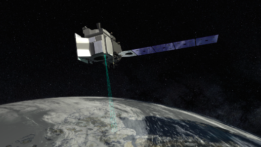
The Advanced Topographic Laser Altimeter System (ATLAS), for measuring elevation, is the only instrument onboard ICESat-2. ATLAS is designed to acquire high resolution measurements of Earth’s surface while also obtaining atmospheric backscatter from molecules, clouds, and aerosols. The overall objectives of ICESat-2 are to quantify the polar ice sheet mass balance to determine contributions to current and recent sea level changes and impacts on ocean circulation, determine the seasonal cycle and topographic character of ice sheet changes, estimate sea ice thickness to examine ice/ocean/atmosphere exchanges of energy, masss and moisture, and measure vegetation canopy height as a basis for estimating large-scale biomass and biomass change. ICESat-2 will provide high quality topographic measurements that allow estimates of ice sheet volume change, key measurements in determining the rate of climate change on Earth. ATLAS receives backscatter from thick clouds, aerosols and molecules in the atmosphere allowing it to measure atmospheric tenuous clouds and blowing snow to provide for atmospheric climate models. These atmospheric measurements are important in climate studies as they extend the data records begun by other Earth observation satellite lidars.
Performance Specifications
ATLAS has a swath width of 17 m, and is able to measure ice-sheet elevation changes to an accuracy of 4 mm per year. For land ice measurements, ATLAS can measure surface elevation changes as little as 0.25 m per year over areas of 100 km2, surface elevation changes with an accuracy of 0.4 m/year along 1 km track segments, and resolution of winter and summer ice-sheet elevation change to 0.1 m at 25 km x 25 km spatial scales. For sea ice measurements, ATLAS can measure monthly surface elevation changes with an uncertainty of 0.03 m along 25 km. ICESat-2 produces elevation measurements that enable the determination of global vegetation height to 3 m accuracy at 1 km spatial resolution in vegetated areas. The backscatter from clouds and aerosols from 14 km altitude to the surface is recorded in an atmospheric channel, which consists of 30m bins in a 14km long column with along track resolution of 280 m.
ICESat-2 is in a near-polar Low Earth Orbit (LEO) at an altitude of 496 km with an orbital inclination of 92° and repeat cycle of 91 days.
Space and Hardware Components
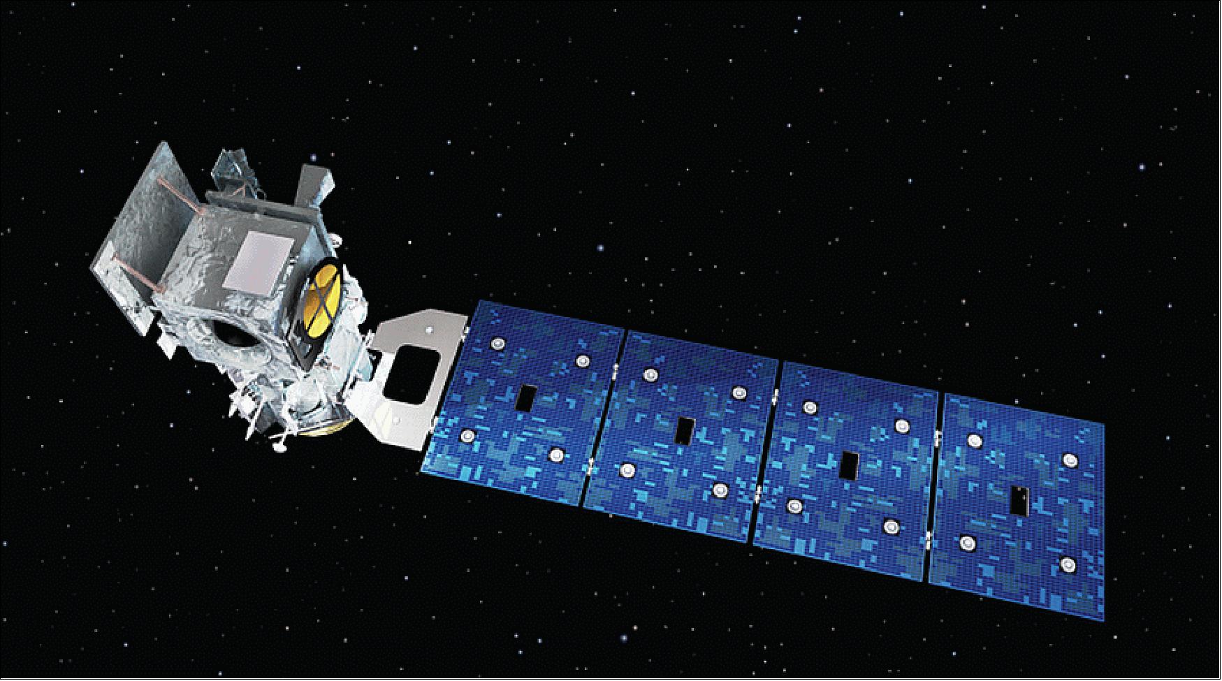
The ICESat-2 spacecraft was built by Northrop Grumman. It is powered by the LEOStar-3 spacecraft bus which also provides orbital control for ATLAS as well as propulsion, navigation, attitude control, thermal control, data storage and handling, and ground communication. The spacecraft has an onboard recorder that stores 580 Gbits/day and is able to downlink data through X-band at a rate of 220 Mbit/s. It has 4 solar panels which produce an average of 1320 Watts to power the spacecraft, with four 22 N thrusters and eight 4.5 N thrusters to maintain the satellite’s orbit, determined through a high-precision GPS receiver and laser ranging.
ICESat-2 (Ice, Cloud and land Elevation Satellite-2)
Spacecraft Launch Mission Status Sensor Complement Ground Segment Preparatory Campaigns References
ICESat-2 is a NASA follow-up mission to ICESat with the goal to continue measuring and monitoring the impacts of the changing environment. The ICESat-2 observatory contains a single instrument, an improved laser altimeter called ATLAS (Advanced Topographic Laser Altimeter System). ATLAS is designed to measure ice-sheet topography, sea ice freeboard as well as cloud and atmospheric properties and global vegetation. The requirements call for a 5-year operational mission with a goal of 7 years. 1) 2) 3) 4) 5) 6) 7)
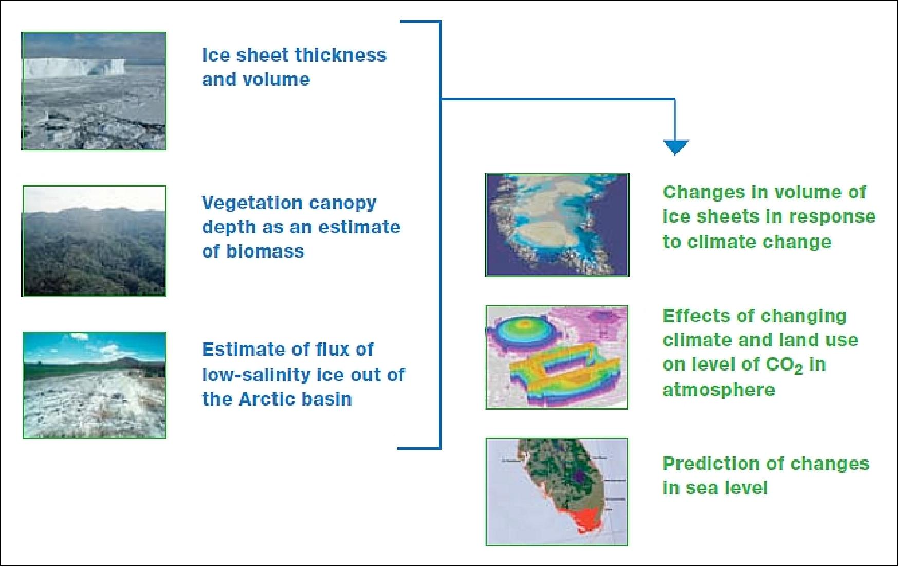
Rational and discussion of mission goals: The mass balance of Earth's great ice sheets and their contributions to sea level are key issues in climate variability and change. The relationships between sea level and climate have been identified as critical subjects of study ib the IPCC (Intergovernmental Panel on Climate Change) assessments, the CCSP (Climate Change Science Program) strategy, and the U.S. IEOS (International Earth Observing System). Because much of the behavior of ice sheets is manifested in their shape, accurate observations of ice elevation changes are essential for understanding ice sheets' current and likely contributions to sea-level rise.
ICESat-2, with high altimetric fidelity, will provide high-quality topographic measurements that allow estimates of ice sheet volume change. High-accuracy altimetry will also prove valuable for making long-sought repeat estimates of sea ice freeboard and hence sea ice thickness change, which is used to estimate the flux of low-salinity ice out of the Arctic basin into the marginal seas. Altimetry is best (and perhaps only) technique for change studies, because sea ice areas and extends have been well observed from space since the 19070s and significant trends have been shown, but there is no such record for sea ice thickness.
As climate change proceeds, continuous measurements of both land-ice and sea-ice volume will be needed to observe trends, update assessments, and test climate models. The altimetric measurement made with the lidar instrument, along with a higher precision gravity measurement (such as GRACE-FO), would optimally characterize changes in ice sheet volume and mass and directly enhance understanding of the ice sheet contribution to sea-level rise. Coupled with the interferometric synthetic aperture radar in the DESDynI mission, the instrumentation would provide a comprehensive data set for predicting changes in Earth's ice sheets and sea ice.
In addition to studies of ice, the proposed instrument could be used to study changes in the large pool of carbon stored in terrestrial biomass. In particular, the proposed lidar could be used to measure canopy depth and thus estimate land carbon storage to aid in understanding the responses of biomass to changing climate and land management. 8) 9) 10)
The overall science objectives are to: 11) 12)
• Quantify the polar ice sheet mass balance to determine contributions to current and recent sea level change and impacts on ocean circulation
• Determine the seasonal cycle of ice sheet changes
• Determine topographic character of ice sheet changes to assess mechanisms driving that change and constrain ice sheet models
• Estimate sea ice thickness to examine ice/ocean/atmosphere exchanges of energy, mass and moisture.
• Measuring vegetation canopy height as a basis for estimating large-scale biomass and biomass change
• Enhancing the utility of other Earth observation systems through supporting measurements.
The instrument will use micro-pulse multi-beam photon-counting approach. Science and ancillary data will be collected, stored on-board and subsequently downlinked to ground stations via an X-band communications link. This link will also include stored housekeeping telemetry. The observatory will also receive and store/execute commands and transmit real-time housekeeping telemetry via an S-band link to the NASA Ground Network.
Spacecraft
The ICESat-2 mission is assigned to NASA/GSFC. The spacecraft is being procured under the GSFC RSDO (Rapid Spacecraft Development Office). In August 2011, NASA selected Orbital ATK, former OSC (Orbital Science Corporation of Dullas, VA, to built the ICESat-2 spacecraft. The contractor is responsible for the design and fabrication of the ICESat-2 spacecraft bus, integration of the government-furnished instrument, satellite-level testing, on-orbit satellite check-out, and continuing on-orbit engineering support. The ICESat-2 spacecraft is being designed, assembled, and tested at Orbital's satellite manufacturing and test facility in Gilbert, Arizona.
ICESat-2 uses the LEOStar-3 platform (used for NASA's Landsat-8, the GeoEye-1 Earth imaging satellite) and is being built and integrated. at the Gilbert, AZ, location of Orbital ATK. 13) 14) 15)
Spacecraft bus | LEOStar-3 |
Spacecraft launch mass, power | 1387 kg, 1.2 kW |
Spacecraft stabilization | 3-axis, zero momentum bias, nadir pointing |
Pointing control | 13.3 arcsec (3σ) |
Orbit determination | High precision GPS receiver and Laser ranging |
Onboard data storage capacity | 704 Gbit at EOL (End of Life) |
Data downlink | X-band, data rate of 220 Mbit/s |
Propulsion | Blowdown hydrazine, four 22 N thrusters and eight 4.5 N thrusters, 158 kg tank capacity |
Mission design life | 3 years with a 5 year goal; 7 years of propellant available |
Project Development Status
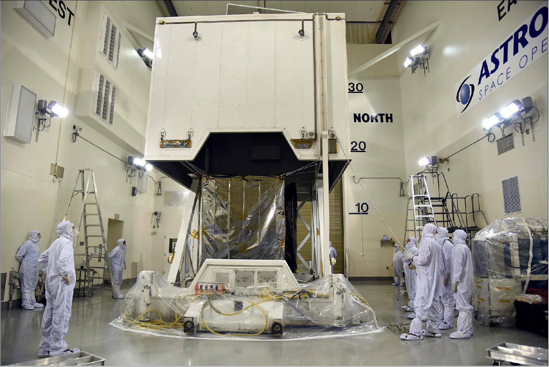
• On 23 June 2018, ICESat-2 engineers at Vandenberg Air Force Base in California successfully finished the final ground-based test of the lasers, which are part of the satellite's sole instrument called the ATLAS (Advanced Topographic Laser Altimeter System). ICESat-2 is scheduled to launch from Vandenberg on Sept. 12, 2018. 16)
- ATLAS was built at NASA's Goddard Space Flight Center in Greenbelt, Maryland, and trucked to a Northrop Grumman facility in Arizona where it was integrated with the spacecraft bus that provides power, navigation and communications. The completed satellite arrived at Vandenberg on June 12.
Note: On June 6, 2018, Northrop Grumman Corporation announced it has closed the acquisition of Orbital ATK Inc. (“Orbital ATK”), a global leader in aerospace and defense technologies. Orbital ATK is now Northrop Grumman Innovation Systems, a new, fourth business sector. 17)
- In the Astrotech Space Operations cleanroom at Vandenberg, the ICESat-2 team tested both the spacecraft and instrument. NASA ICESat-2 launch integration manager John Satrom reports that the data from these tests have been reviewed and everything is normal.
- Meanwhile at Vandenberg's Space Launch Complex 2 along the Pacific coast, crews from United Launch Alliance are assembling the Delta II rocket that will launch ICESat-2 into space. The first and second stage, the interstage connecting them, and four solid rocket motors are in place. The ICESat-2 mission will mark the final launch for the Delta II, which will then be retired.
- After the successful completion of another round of “aliveness” tests turning on the satellite and instrument at the end of July, the ICESat-2 payload is scheduled to head to the launch pad in late August, according to Satrom.
• February 28, 2018: The ATLAS (Advanced Topographic Laser Altimeter System) instrument, which was designed, built and tested at NASA's Goddard Space Flight Center in Greenbelt, Maryland, arrived in Gilbert, Arizona, at Orbital ATK's facility on Feb. 23, where it will be joined with the spacecraft structure. To deliver the instrument safely to the spacecraft for assembly and testing, the ATLAS team developed special procedures for packing, transporting and monitoring the sensitive hardware. 18)
- "There was a lot of care and feeding that went with ATLAS along the road," said Kathy Strickler, ATLAS integration and test lead.
- The trip followed a successful series of tests, designed to ensure the ATLAS instrument will function in the harsh environment of space. After the instrument passed those tests, including some in a thermal vacuum chamber, engineers inspected ATLAS to make sure it was clean and in the correct travel configuration. Then, they attached probes to the instrument that would check for vibrations as well as temperature and humidity.
- "These probes tracked what ATLAS actually sensed when going over road bumps, and what ATLAS felt as far as temperature and humidity," said Jeffrey Twum, the ATLAS transport lead.
- The team then wrapped the instrument - about the size of a Smart Car - in two layers of anti-electrostatic discharge film, to prevent any shocks en route. With its protections in place, a crane lifted ATLAS into a transporter container. The team bolted it to a platform supported by a series of wire-rope coils used to soften the ride, and the cover of the transporter was fastened shut, sealing up the cargo.
- The 2,000-mile trip took four and a half days. The ATLAS instrument is now at Orbital ATK, where engineers will attach it to the spacecraft and conduct additional testing. Then, the complete satellite will be repacked and trucked to its last stop before low-Earth orbit: Vandenberg Air Force Base in California.
• August 16, 2017: Lasers that will fly on NASA’s ICESat-2, are about to be put to the test at the agency’s Goddard Space Flight Center in Greenbelt, Maryland. 19)
- The sole ICESat-2 instrument, ATLAS (Advanced Topographic Laser Altimeter System) will measure the elevation of ice sheets, sea ice and glaciers by sending fast-firing laser pulses to the surface and timing how long it takes individual photons to return. With a scheduled launch date of 2018, the instrument now faces several months of testing at Goddard in which engineers will ensure it is ready to operate in the harsh environment of space. This is an intermediate stage of ICESat-2’s testing regimen, and will focus on the flight lasers.
- Starting this fall, ATLAS will go into a test chamber at Goddard where engineers simulate the vacuum of space and can dial temperatures up to 50 C to - 30 C. Engineers will also turn on the two lasers — one primary and one backup — at different power levels to ensure they function correctly, said Anthony Martino, ATLAS instrument scientist at NASA Goddard. One test will include putting the instrument through its paces at different temperatures and taking pictures of the laser pulses to ensure they form a smooth, consistent circle, Martino said, with no rough edges, or dark or light spots.
- “When it’s well behaved like that, it’s much easier to analyze the results that we’ll get,” he said. Other tests involve using mirrors to reflect the laser back into the detector portions of the instrument — but only after decreasing the strength of the beam of light by 13 orders of magnitude (about 10 trillion times), to simulate the weakening of the laser beam as it is scattered by the atmosphere, bounces off Earth and returns.
• September 2016: ICESat-2 Technical Status Summary. 20)
Beyond the ATLAS instrument, all other ICESat‐2 systems are nearing completion including spacecraft, launch vehicle, algorithms, operations planning, and ground systems.
- The mission requirements remain intact through the ongoing flight Laser002 repair.
- The ATLAS management and engineering team has crafted and is implementing a conservative plan to address the recent Laser002 optical slab fracture.
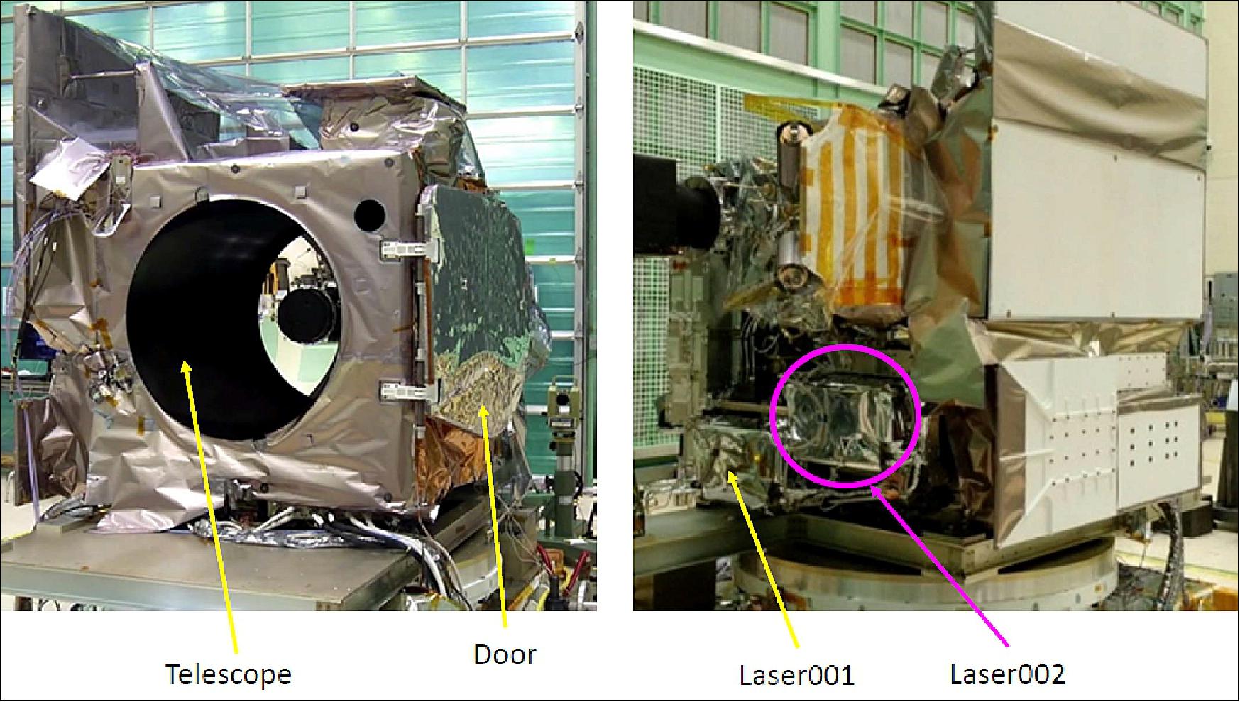
ATLAS Instrument – Technical Issue with Laser002
• The ATLAS instrument completed integration and testing campaigns for EMI/EMC (Electromagnetic Interference/Electromagnetic Compatibility) and Vibration
• During Thermal Vacuum (TVac) testing, Laser002 (the second of two onboard flight lasers) exhibited a performance anomaly
- During one of several start-ups, the Laser002 pre-amplifier, amplifier, and SHG (Second Harmonic Generator) energy monitors dropped suddenly
- After the drop, the pre-amplifier, amplifier, and SHG energy levels increased, and started to oscillate
- Subsequent turn-ons of Laser002 (post-anomaly) energy monitors and ATLAS SPD (Start Pulse Detector) energy readings slowly varied, eventually stabilizing at lower than nominal values (~70 to 80% of nominal)
• Ongoing investigation and repair of Laser002
- The Thermal Vacuum testing was suspended and Laser002 was de-integrated from ATLAS and returned to the vendor, Fibertek
- Fibertek completed disassembly and initial inspection of Laser002 pre-amplifier assembly
- The crystal optical slab within the pre-amplifier assembly fractured towards the center at a point where thermal stress is low indicating proximate cause was mechanical stress from mount clamp assembly (~1cm from pump face)
- Observed uneven intermetallic growth on mount and clamp surface indicating poor contact between these surfaces
- Completed X-ray tomography of Laser002 pre-amplifier assembly and observed non-uniform intermetallic growth between slab and clamp/mount surfaces
- Ongoing review of mount re-work/re-design options with Fibertek.
• Feb. 18, 2016: ICESat-2 passed its Mission CDR (Critical Design Review)! Now, on to building and testing software and hardware for flight. 21)
• Jan. 17, 2016: ICESat-2 passed its Instrument Critical Design Review! The project is now moving full-speed ahead to Mission CDR and instrument I&T start.
• Dec. 10, 2015: NASA engineers tested the ATLAS instrument's pinpoint accuracy. ATLAS (Advanced Topographic Laser Altimeter System) will send laser pulses to the ground about 480 km below and then catch the handful of photons that bounce off the surface and return to its telescope mirror. There's very little margin for error when it comes to individual photons hitting on individual fiber optics - so this November, engineers conducted a series of tests on the ground, to ensure that they could hit that mark when ICESat-2 is in orbit. 22)
- This is the first time Goddard has built an automatically correcting and steering mechanism like this for flight. It was necessary for ATLAS, however, because both the receiver's field-of-view and the laser beam diameter are significantly smaller than on previous instruments, so there is less room for the laser to drift off-target. So the AMCS (Alignment Monitoring and Control System) team spent several weeks in November 2015 testing the steering mechanism and the software that controls it.
• February 2015: A NASA team tested part of the ATLAS instrument in a temperature-controlled vacuum chamber at Goddard, ensuring that its interconnected components worked together and functioned as expected. 23)
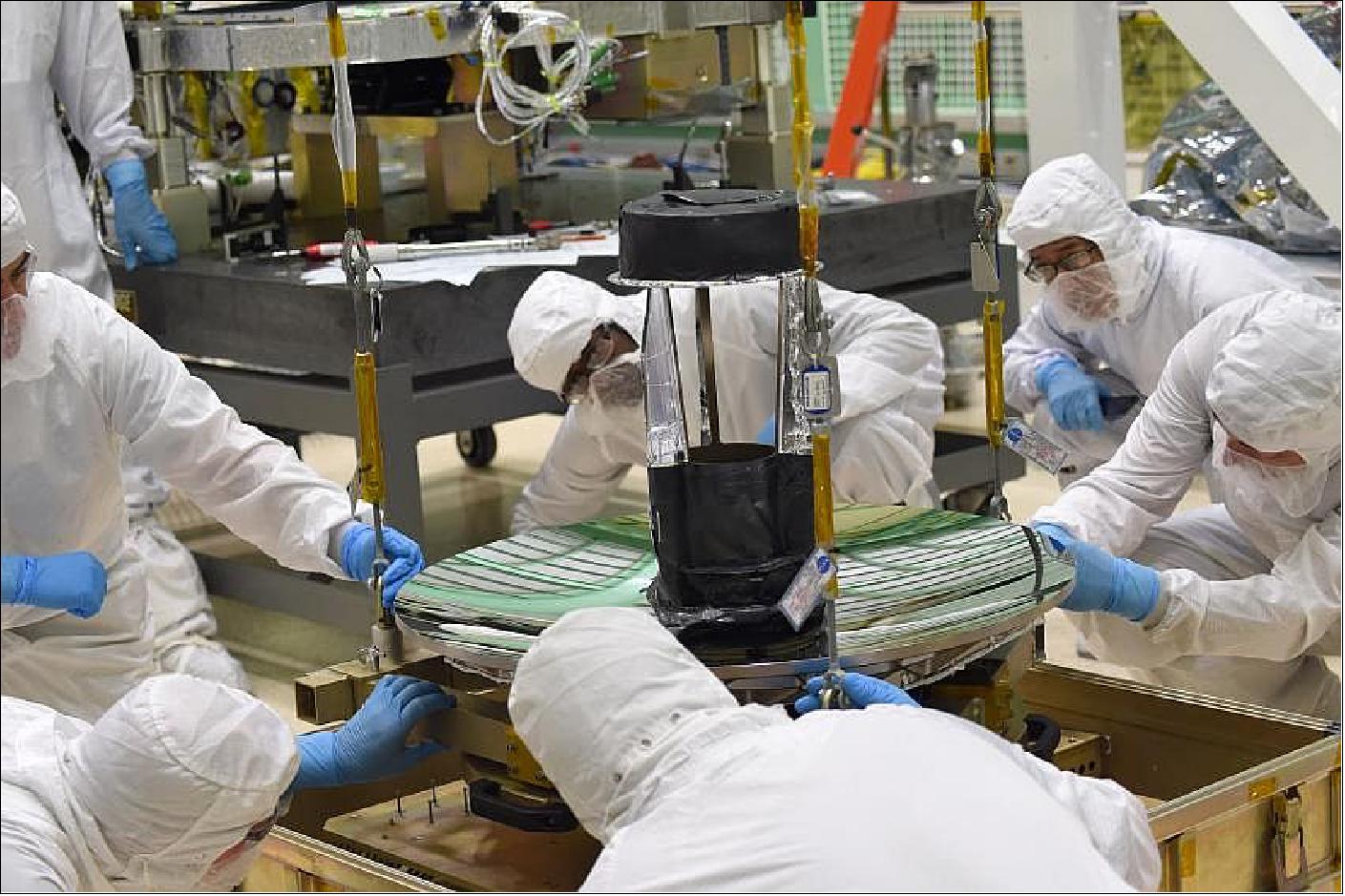
• November 3, 2014: Engineers at NASA/GSFC fitted the mirrored telescope of ICESat-2 into its place. In a Goddard cleanroom, teams are working in parallel on two sections of ATLAS: the box structure, which holds electronics that control the instrument, and the optical bench, which supports the instrument's lasers, mirrors, and the 0.8 m, 20.8 kg beryllium telescope that collects light. 24)
- Each ATLAS laser pulse contains more than 200 trillion photons, but only a dozen or so return to the telescope, where they're sent via optical fibers to the instrument's detectors. To catch those few photons, the telescope and its associated equipment, called the RTA (Receiver Telescope Assembly), need to align perfectly to the laser.
• Sept. 1, 2014: Due to cost overruns, the launch of ICESat-2 has slipped to June 2018. ICESat-2’s overrun was driven primarily by technical difficulties with the ATLAS (Advanced Topographic Laser Altimeter System) instrument. 25)
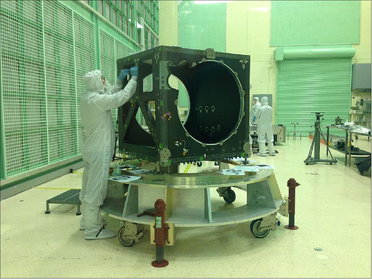
• May 2014: The box structure of the ATLAS instrument was delivered to a clean room at NASA/GSFC (Figure 66). A team of 250 engineers, fabricators and scientists has now started the official integration and testing stage of the laser instrument (Ref. 77).
• February 18, 2014: ICESat-2 passed its Mission Critical Design Review! Now, on to building and testing software and hardware for flight.
• January 17, 2014: ICESat-2 passed its Instrument CDR (Critical Design Review)! The project is now moving full-speed ahead to Mission CDR and instrument I&T start.
• In December 2013, NASA notified Congress of expected budget increases ($200 million overrun) on the ICESat-2 mission. NASA is required by law to inform Congress when a mission appears likely to overrun its approved budget by more than 15%. This may cause possible launch delays. 26)
• Sept. 6, 2013: ICESat-2 passed its Ground Systems CDR (Critical Design Review). An independent review board met Sept. 3-5 , 2013at Goddard Space Flight Center in Greenbelt, MD, to examine details of the entire design of the mission's ground system, including the MOC (Mission Operations Center), the ISF (Instrument Support Facility), and the Science Investigator-led Processing System.
• The ICESat-2 mission was assigned Phase C status on December 17, 2012.
• The ICESat-2 project passed instrument PDR (Preliminary Design Review) on Nov. 18, 2011.
• The ICESat-2 team passed the SRR (System Requirements Review) on May 25, 2011.
• The ICESat-2 team passed the ISRE (Instrument System Requirements Review) on December 1, 2010.
• The ICESat-2 team passed the Key Decision Point A (KDP-A) review at HQ on December 11, 2009. Since then the project started officially in Phase A.
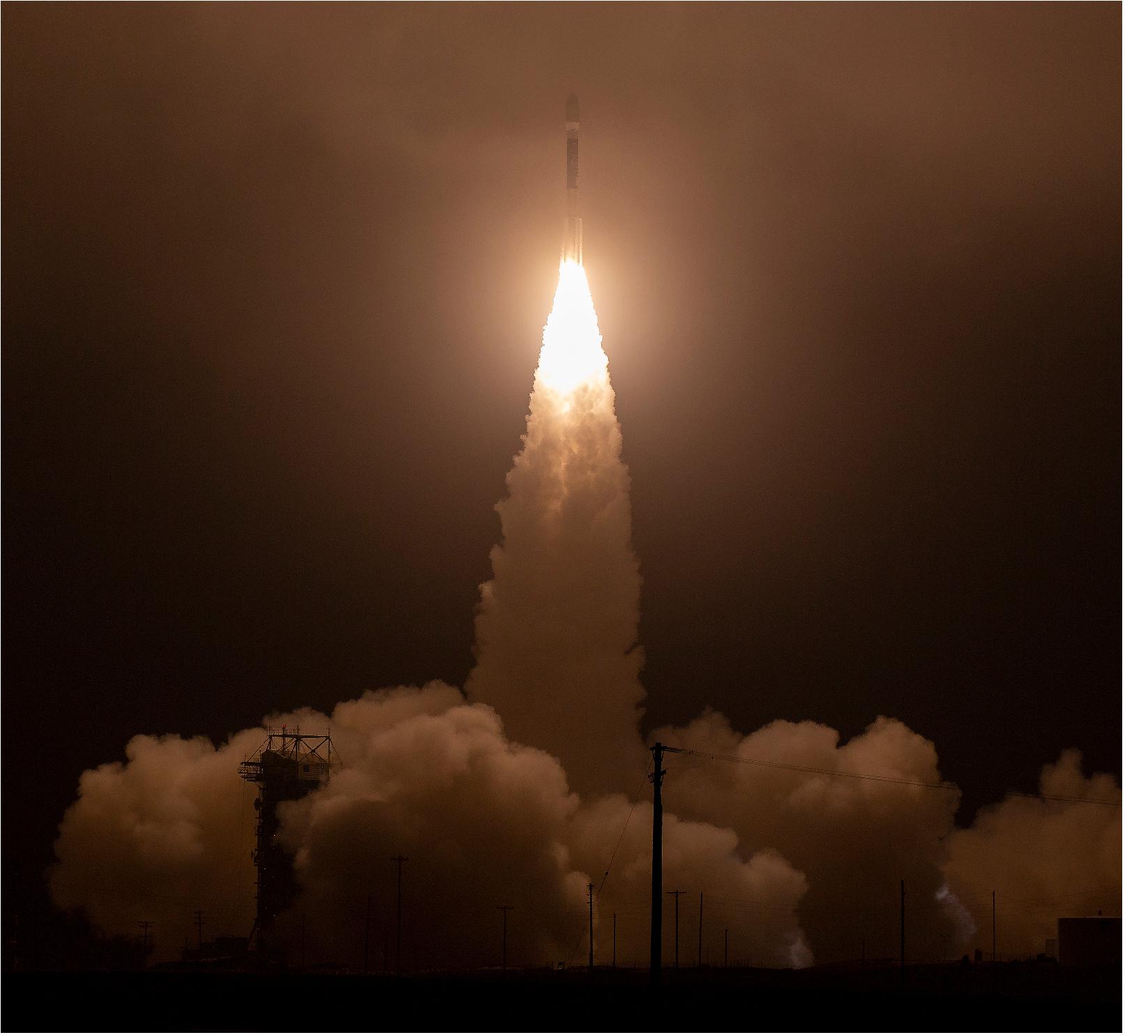
Launch: The ICESat-2 spacecraft was launched on 15 September 2018 (13:02 UTC) from VAFB, CA (Space Launch Complex -2W) on a Delta-II 7420-10 vehicle configuration. The launch service provider was ULA (United Launch Alliance). 27) 28) 29)
This marked the final launch of the Delta II rocket series. ULA's Delta II rocket has provided dependable access to space for the U.S. military, NASA and commercial clients for nearly 30 years, launching 154 times since its debut on Feb. 14, 1989. The lasting legacy of the Delta II extends from creating modern GPS navigation on Earth to roving the surface of Mars.
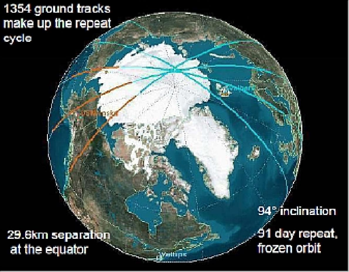
Orbit: Near polar LEO frozen orbit, altitude =496 km, inclination = 92º, repeat cycle of 91 days with subcycles of 29, 29, and 33 days (Figure 9).
The Secondary Payloads on IceSat-2
In addition to ICESat-2, this mission includes four cubesats that will launch from dispensers mounted to the Delta II’s second stage.
• ELFIN (Electron Losses and Fields Investigation), a pair of 3U CubeSats of UCLA (University of California Los Angeles). 30)
• SurfSat (Surface charging Satellite), a 2U CubeSat mission developed at the UCF (University of Central Florida), Orlando, FL.
• CP-7 (CalPoly-7) or DAVE (Damping And Vibrations Experiment), a 1U CubeSat, a collaboration of Northrop Grumman Aerospace Systems and CalPoly.
Mission Status
• June 28, 2022: Arctic sea ice has lost about a third of its volume since 2003. At the other pole, new glacial lakes were discovered deep below the surface of Antarctic ice. At latitudes in between, changing water levels in reservoirs revealed human influences. 31)
- Those are just a few of the 100-plus new findings made with precise height data from the 12 trillion laser measurements collected from NASA’s Ice, Cloud and land Elevation Satellite-2 (ICESat-2).
- Since its September 2018 launch, ICESat-2 has gathered data and inspired research on our changing Earth – ranging from ice to tropical beaches, boreal forests to urban areas. Before launch, mission science team members talked of what they hoped it would help us understand. Now, the mission has the green light to continue operation after successfully completing its three-year primary mission, and these ice scientists share what it has revealed.
• February 10, 2022: NASA has awarded the Ice, Cloud, and land Elevation-2 (ICESat-2) Mission Operations Center Support contract to Northrop Grumman Systems Corporation of Dulles, Virginia. 32)
- This is a cost-plus award-fee contract that includes a nine-month base period and four one-year options with a total contract value of $33,348,387. The four-year, nine-month period of performance begins Monday, Feb 14. The work will be performed at the contractor’s facility in Dulles, Virginia.
- Under this follow-on contract, Northrup Grumman Space Systems will continue to provide ICESat-2 mission operations; data processing and analysis; mission planning; commanding; Solid State Recorder management and monitoring; orbit and attitude determination and control; flight software maintenance; anomaly identification and resolution; and delivery of science and engineering data products.
- NASA’s ICESat-2 mission, launched in 2018, allows scientists to investigate why and how much of the frozen parts of our world are changing as a result of climate change. All ICESat-2 data are housed and managed at the NASA National Snow and Ice Data Center Distributed Active Archive Center (NSIDC DAAC).
• July 7, 2021: From above, the Antarctic Ice Sheet might look like a calm, perpetual ice blanket that has covered Antarctica for millions of years. But the ice sheet can be thousands of meters deep at its thickest, and it hides hundreds of meltwater lakes where its base meets the continent’s bedrock. Deep below the surface, some of these lakes fill and drain continuously through a system of waterways that eventually drain into the ocean. 33)
- Now, with the most advanced Earth-observing laser instrument NASA has ever flown in space, scientists have improved their maps of these hidden lake systems under the West Antarctic ice sheet—and discovered two more of these active subglacial lakes.
- The new study provides critical insight for spotting new subglacial lakes from space, as well as for assessing how this hidden plumbing system influences the speed at which ice slips into the Southern Ocean, adding freshwater that may alter its circulation and ecosystems.
- NASA's ICESat-2 (Ice, Cloud and land Elevation Satellite-2) allowed scientists to precisely map the subglacial lakes. The satellite measures the height of the ice surface, which, despite its enormous thickness, rises or falls as lakes fill or empty under the ice sheet.
- The study, published July 7 in Geophysical Research Letters, integrates height data from ICESat-2’s predecessor, the original ICESat mission, as well as the European Space Agency’s satellite dedicated to monitoring polar ice thickness, CryoSat-2. 34)
- Hydrology systems under the Antarctic ice sheet have been a mystery for decades. That began to change in 2007, when Helen Amanda Fricker, a glaciologist at Scripps Institution of Oceanography at the University of California San Diego, made a breakthrough that helped update classical understanding of subglacial lakes in Antarctica.
- Using data from the original ICESat in 2007, Fricker found for the first time that under Antarctica’s fast flowing ice streams, an entire network of lakes connect with one another, filling and draining actively over time. Before, these lakes were thought to hold meltwater statically, without filling and draining.
- “The discovery of these interconnected systems of lakes at the ice-bed interface that are moving water around, with all these impacts on glaciology, microbiology, and oceanography—that was a big discovery from the ICESat mission,” said Matthew Siegfried, assistant professor of geophysics at Colorado School of Mines, Golden, Colo. and lead investigator in the new study. “ICESat-2 is like putting on your glasses after using ICESat, the data are such high precision that we can really start to map out the lake boundaries on the surface.”
- Scientists have hypothesized subglacial water exchange in Antarctica results from a combination of factors, including fluctuations in the pressure exerted by the massive weight of the ice above, the friction between the bed of the ice sheet and the rocks beneath, and heat coming up from the Earth below that is insulated by the thickness of the ice. That’s a stark contrast from the Greenland ice sheet, where lakes at the bed of the ice fill with meltwater that has drained through cracks and holes on the surface.
- To study the regions where subglacial lakes fill and drain more frequently with satellite data, Siegfried worked with Fricker, who played a key role in designing the way the ICESat-2 mission observes polar ice from space.
- Siegfried and Fricker’s new research shows that a group of lakes including the Conway and Mercer lakes under the Mercer and Whillans ice streams in West Antarctica are experiencing a draining period for the third time since the original ICESat mission began measuring elevation changes on the ice sheet’s surface in 2003. The two newly found lakes also sit in this region.
- In addition to providing vital data, the study also revealed that the outlines or boundaries of the lakes can change gradually as water enters and leaves the reservoirs.
- “We're really mapping out any height anomalies that exist at this point,” Siegfried said. “If there are lakes filling and draining, we will detect them with ICESat-2.”
'Helping Us Observe' Under the Ice Sheet
- Precise measurements of basal meltwater are crucial if scientists want to gain a better understanding of Antarctica’s subglacial plumbing system, and how all that freshwater might alter the speed of the ice sheet above or the circulation of the ocean into which it ultimately flows.
- An enormous dome-shaped layer of ice covering most of the continent, the Antarctic ice sheet flows slowly outwards from the central region of the continent like super thick honey. But as the ice approaches the coast, its speed changes drastically, turning into river-like ice streams that funnel ice rapidly toward the ocean with speeds up to several meters per day. How fast or slow the ice moves depends partly on the way meltwater lubricates the ice sheet as it slides on the underlying bedrock.
- As the ice sheet moves, it suffers cracks, crevasses, and other imperfections. When lakes under the ice gain or lose water, they also deform the frozen surface above. Big or small, ICESat-2 maps these elevation changes with a precision down to just a few inches using a laser altimeter system that can measure Earth’s surface with unprecedented detail.
- Tracking those complex processes with long-term satellite missions will provide crucial insights into the fate of the ice sheet. An important part of what glaciologists have discovered about ice sheets in the last 20 years comes from observations of how polar ice is changing in response to warming in the atmosphere and ocean, but hidden processes such as the way lake systems transport water under the ice will also be key in future studies of the Antarctic Ice Sheet, Fricker said.
- “These are processes that are going on under Antarctica that we wouldn't have a clue about if we didn't have satellite data,” Fricker said, emphasizing how her 2007 discovery enabled glaciologists to confirm Antarctica’s hidden plumbing system transports water much more rapidly than previously thought. “We've been struggling with getting good predictions about the future of Antarctica, and instruments like ICESat-2 are helping us observe at the process scale.”
'A Water System That Is Connected to the Whole Earth System'
- How freshwater from the ice sheet might impact the circulation of the Southern Ocean and its marine ecosystems is one of Antarctica’s best kept secrets. Because the continent’s subglacial hydrology plays a key role in moving that water, Siegfried also emphasized the ice sheet’s connection to the rest of the planet.
- “It's not just the ice sheet we're talking about,” Siegfried said. “We're really talking about a water system that is connected to the whole Earth system.”
- Recently, Fricker and another team of scientists explored this connection between freshwater and the Southern Ocean—but this time by looking at lakes near the surface of an ice shelf, a large slab of ice that floats on the ocean as an extension of the ice sheet. Their study reported that a large, ice-covered lake collapsed abruptly in 2019 after a crack or fracture opened from the lake floor to the base of Amery Ice Shelf in East Antarctica.
- With data from ICESat-2, the team analyzed the rugged change on the landscape of the ice shelf. The event left a doline, or sinkhole, a dramatic depression of about four square miles (about 10 km2), or more than three times the size of New York City's Central Park. The crack funneled nearly 200 billion gallons of freshwater from the surface of the ice shelf into the ocean below within three days.
- During the summer, thousands of turquoise meltwater lakes adorn the bright white surface of Antarctica’s ice shelves. But this abrupt event occurred in the middle of the winter, when scientists expect water on the surface of the ice shelf to be completely frozen. Because ICESat-2 orbits Earth with exactly repeating ground tracks, its laser beams can show the dramatic change in the terrain before and after the lake drained, even during the darkness of polar winter.
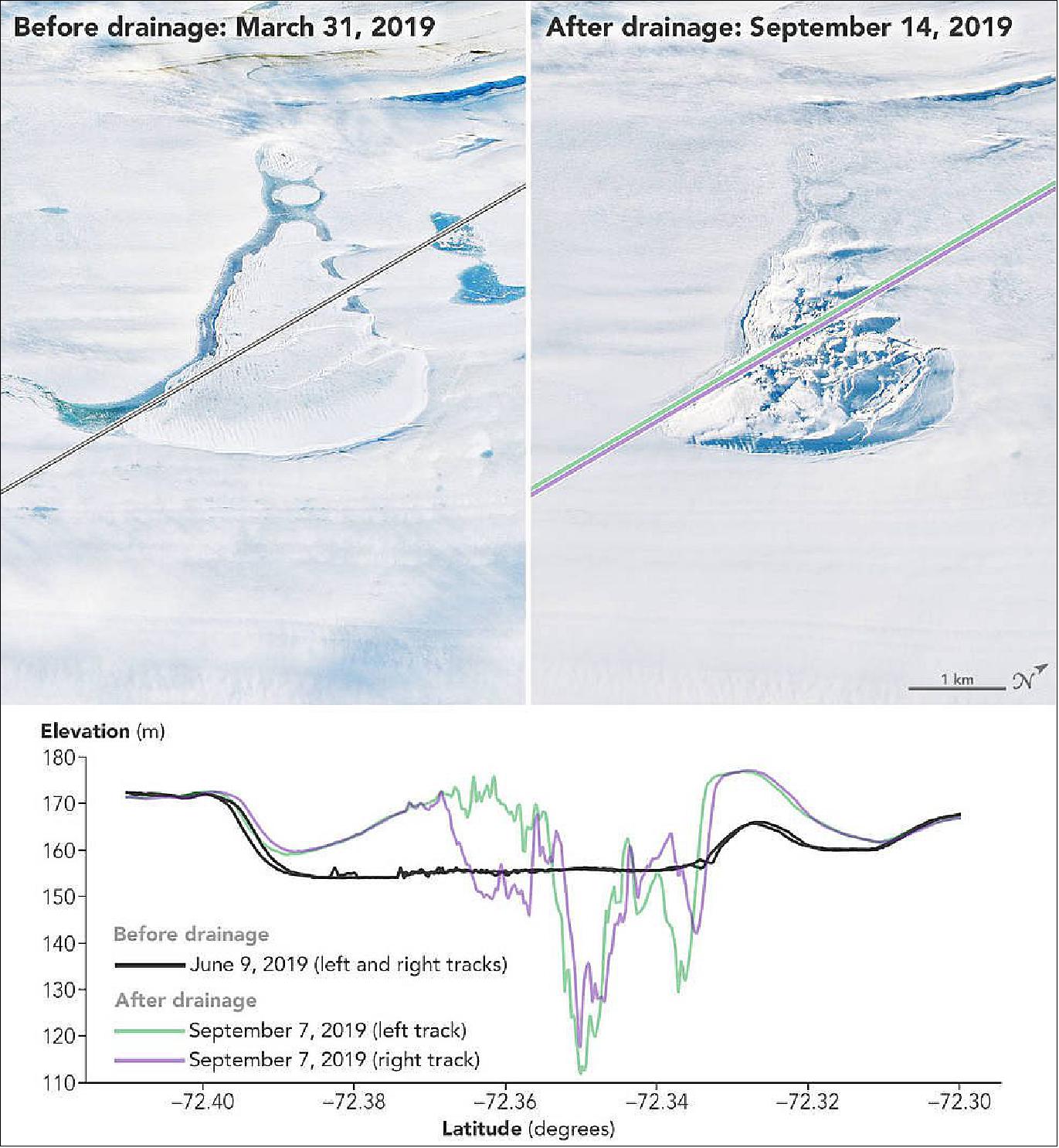
- Roland Warner, a glaciologist with the Australian Antarctic Program Partnership at the University of Tasmania, and lead author of the study, first spotted the scarred ice shelf in images from Landsat 8, a joint mission of NASA and the U.S. Geological Survey. The drainage event was most likely caused by a hydrofracturing process in which the mass of the lake’s water led to a surface crack being driven right through the ice shelf to the ocean below, Warner said.
- “Because of the loss of this weight of water on the surface of the floating ice shelf, the whole thing bends upwards centered on the lake,” Warner said. “That's something that would have been difficult to figure out just staring at satellite imagery.”
- Meltwater lakes and streams on Antarctica’s ice shelves are common during the warmer months. And because scientists expect these meltwater lakes to be more common as air temperatures warm, the risk of hydrofracturing could also increase in coming decades. Still, the team concluded it’s too early to determine whether warming in Antarctica’s climate caused the demise of the observed lake on Amery Ice Shelf.
- Witnessing the formation of a doline with altimetry data was a rare opportunity, but it is also the type of event glaciologists need to analyze in order to study all of the ice dynamics that are relevant in models of Antarctica.
- “We have learned so much about ice sheet dynamic processes from satellite altimetry, it is vital that we plan for the next generation of altimeter satellites to continue this record,” Fricker said.
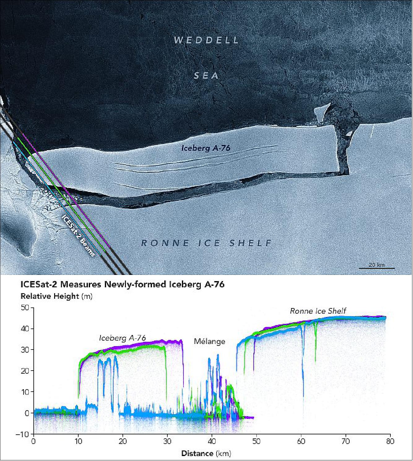
• June 3, 2021: In terms of size, only one iceberg can reign supreme at a time—a position recently held by Iceberg A-76 in the Weddell Sea. When the berg calved from Antarctica’s Ronne Ice Shelf in May 2021, it became the largest iceberg floating anywhere in the world. 35)
- Antarctica’s ice shelves are famous for cutting loose some mammoth icebergs. The largest are usually tabular icebergs, named for their table-like shape with steep sides and large, flat tops. Iceberg A-76 represents a classic tabular iceberg, but as the elevation profile of Figure 14 shows, even this picture-perfect berg is not perfectly flat.
- “Ice is a somewhat strange material,” said Ted Scambos, a research glaciologist at the University of Colorado. “We’re not used to its particular combination of strength, brittleness, and bendy-ness.”
- The profile of Figure 14 was acquired with the Advanced Topographic Laser Altimeter System (ATLAS) on NASA’s Ice, Cloud, and land Elevation Satellite 2 (ICESat-2). ATLAS is a photon-counting lidar that sends pulses of laser light toward Earth and precisely times each photon’s round-trip journey as it bounces off a surface and returns to the sensor. From this information scientists can derive the height of the surface hit by the photon.
- The beams first pass over relatively flat open water before reaching the leading edge of the iceberg, where the elevation profiles begin to differ. Notice the jagged texture of the ice where the blue beam clips the berg’s western edge. The irregular shape was created when the berg was still attached to the ice shelf and flowing through a zone known as a shear margin. As “fast” flowing ice pushed past the rocky ice-covered peninsula, powerful stresses caused the ice to crumple.
- The green and purple beams reveal the more typical profile of a tabular iceberg. Notice that the seaward edge appears lower. For 21 years—since the last time an iceberg calved from the Ronne Ice Shelf—melting has taken a toll on the exposed front edge. Its underside has likely been eroded by seawater carving it from below it during thousands of tidal cycles.
- By comparison, the iceberg’s fresh interior edge is higher, standing about 35 meters (100 feet) above sea level. That means the berg would be about 280 meters thick, including most of the iceberg that exists below the water line and out of sight.
- There are other intricacies visible as well. The interior edge shows a classic steep face, with a series of crests and troughs on the iceberg’s surface as you move away from the edge. Models have shown that this is how the ice of an iceberg like A-76 should respond after breaking from an ice shelf.
- “At the very first instant and a few days after a sharp break, the fresh edge has one shape based on the ‘rigid’ response of the ice,” Scambos said. “But the ice slowly responds to the stress and bends over the course of days to a slightly different shape.”
- The profile also exposes mélange—a mixture of broken ice floating on the sea surface—before rising steeply at the newly exposed face of the Ronne Ice Shelf. The blue beam dips sharply (and the green beam to a lesser extent) at the location of a rift on the ice shelf along the shear margin—in a similar location to a rift that helped spawn Iceberg A-76.
- According to Christopher Shuman, a University of Maryland, Baltimore County, glaciologist based at NASA’s Goddard Space Flight Center: “The rest of the Ronne front now bears watching to see when it will respond to the calving of A-76.”
- By June 2021, the iceberg had broken into three named pieces (A-76A, A-76B, and A-76C) and lost its position as the world’s largest iceberg. Iceberg A-23A, adrift since 1986 and currently measuring about 1,500 square miles (4,000 km2), regained the title.
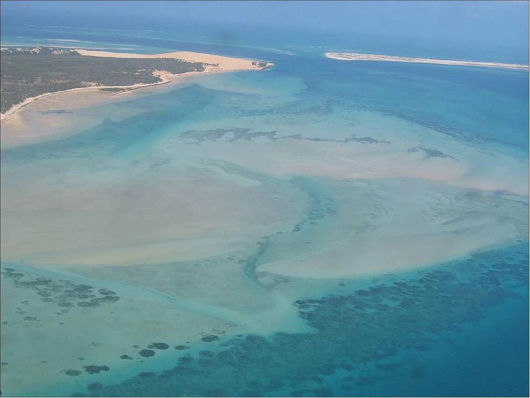
• April 30, 2021: The shallow waters around islands and continental coastlines are important for human activities and for the health of many marine species. Yet these areas are constantly evolving and notoriously challenging and time-intensive to map. For several years, remote sensing scientists have worked to change that paradigm. A recent study led by NASA-funded researchers shows how it might be done with freely available satellite data and cloud computing. 36)
- For centuries, marine surveyors relied on shipborne tools—first sounding lines, then sonar—to decipher the depth and shape of the seafloor, or bathymetry. Starting with U.S. Landsat satellites in the 1970s and more recently with European Sentinel satellites, researchers have been slowly developing ways to derive bathymetric information from satellite images.
- Different wavelengths of light penetrate water to differing depths, with shorter wavelengths (such as blue and green) penetrating farther than longer wavelengths (near infrared, shortwave infrared). When water is clear and the seafloor is bright, scientists can estimate depth by measuring the amount of reflectance observed by a satellite and then modeling how far the light should penetrate. 37)
- In 2021, Nathan Thomas and Lola Fatoyinbo of NASA’s Goddard Space Flight Center, along with colleagues from three countries, took another step by mating ICESat-2 measurements with images from Copernicus Sentinel-2 to derive bathymetry at better resolution. The team mapped the shallows down a depth of 26 meters (85 feet) around Biscayne Bay in Florida, the Gulf of Chania in Crete, and the island of Bermuda.
- Thomas and colleagues compared their satellite-derived bathymetry with maps made from traditional topographic surveys, multibeam sonar, and nautical soundings. Their new maps had a resolution of 10 meters, improving upon the current 115-meter resolution dataset for Crete and the 30- to 90-meter datasets for Florida and Bermuda. The existing data for Florida and Bermuda are composites of lots of sources spanning 63 years, while the ICESat-2/Sentinel-2 maps offer a contemporary assessment of underwater structure.
- “Nearshore, shallow-water bathymetry is so important to both society and the natural environment, but openly available information on sub-aquatic structure is uncommon, particularly at high spatial resolutions,” said Thomas. “We were able to improve upon freely available datasets in both detail and imaging period with wall-to-wall maps of nearshore bathymetry at 10-meter resolution.”
- A key part of the effort was the use of open-source data, cloud computing, and tools like Google Earth Engine. “As GEE is an open platform, it gives us a means through which we can share our approach,” Thomas noted. “Others can use our methods and code in a stable computing environment and repeat our work.”
- For island nations and coastal states with limited funds and limited access to equipment, open-source, satellite-based bathymetric maps could be particularly useful. Reliable mapping is important for ship navigation, the development and protection of coastal infrastructure, the placement of aquaculture facilities, and monitoring of nearshore habitat. Even in more industrialized areas, satellite mapping could provide updated, cost-effective seafloor views in areas that change rapidly.
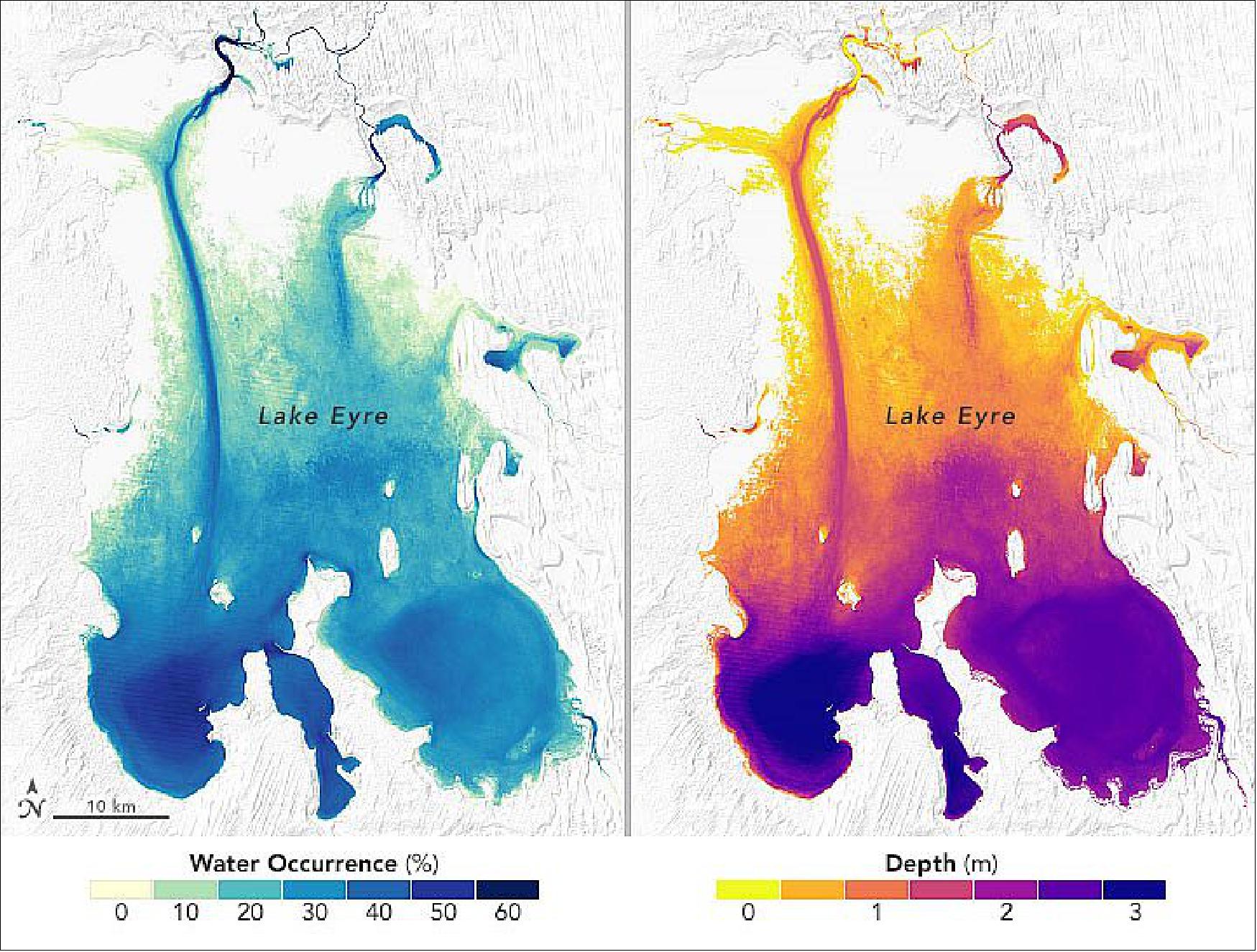
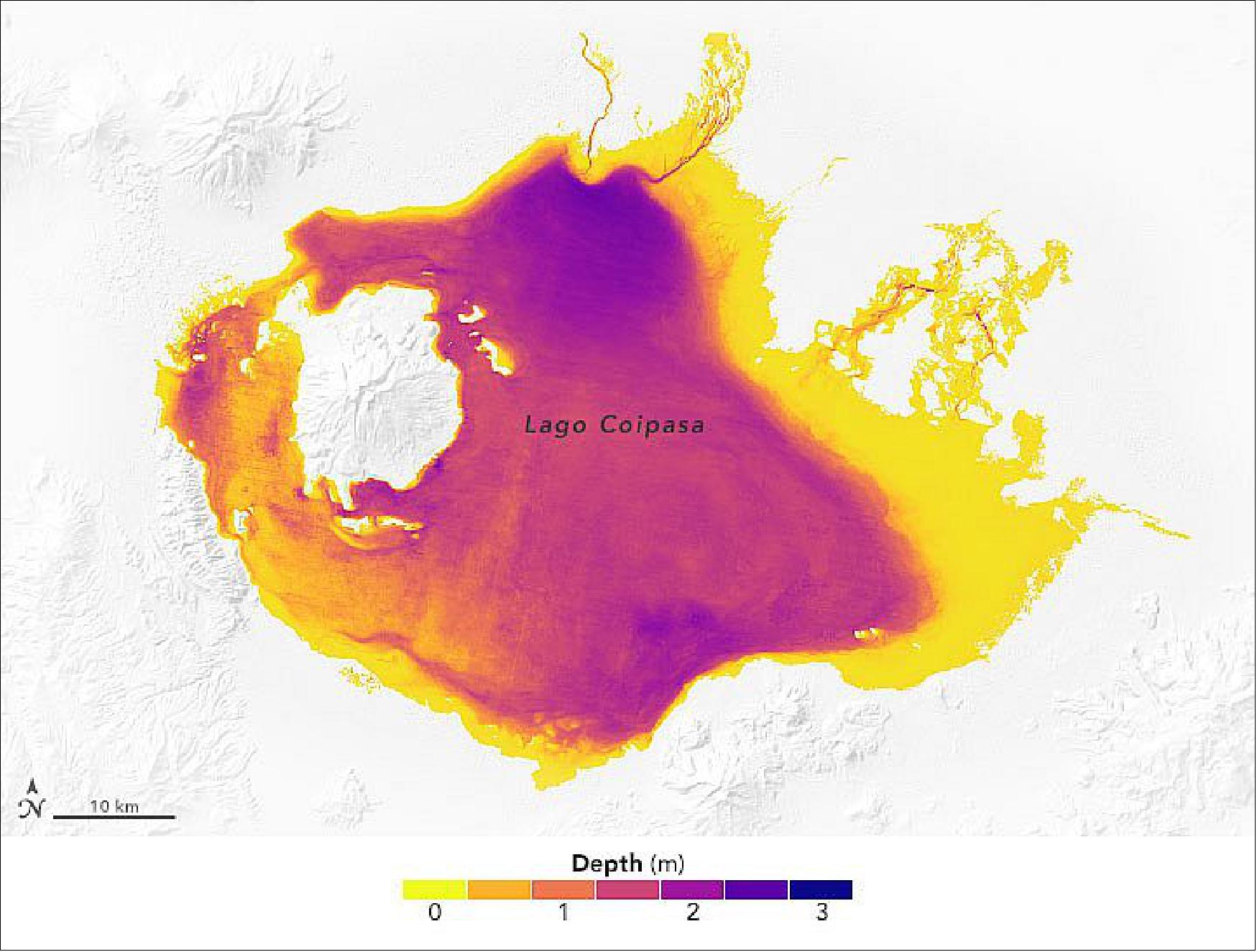
• April 27, 2021: Lakes rarely have uniform depth. They contain dips and bumps across their floors that affect the amount of water they can hold. Traditionally, mapping the bottom of a lake has been done by deploying instruments from boats and ships. But that method is most useful for lakes that are easy to access, important to navigation, or flooded often. 38)
- Now researchers have generated a new technique to measure the depth of some of the most isolated, shallow lakes. Ephemeral lakes usually only fill after heavy seasonal rains or when a passing tropical cyclone drenches the landscape. Scientists from Israel and Australia recently used NASA satellite data to map the shape and depth (bathymetry) of such lakes in deserts.
- By knowing the shapes of lake beds in dry regions, researchers can better estimate the amount of water stored in such basins and then improve water management. They also can reconstruct past climates when the lakes may have been fuller.
- “Desert lakes are used sometimes as water resources, and they are a home to a large diversity of species, relying on flood water to arrive,” said Moshe (Koko) Armon, a graduate student studying hydrology at the Hebrew University of Jerusalem. “To understand the amount of water in a lake when it is flooded, we need to know the shape of its floor in detail and with the best resolution.”
- Armon and colleagues mapped the largest shallow desert lake in the world, Lake Eyre, which spans 9,300 km2 (3,600 square miles) in Australia. While Lake Eyre tends to receive some water each year, the full area is flooded just a few times per century, according to Tim Cohen, a study co-author from Wollongong University. Flood waters help bring abundant vegetation, as well as birds, fish, and amphibians, to these vast water holes.
- “Desert lakes are filled rather quickly by floods, but they empty quite slowly mainly because of evaporation,” said Armon. “The regions holding water for the longest time are the deepest parts of the lake.”
- Armon said a next step in this research would be to look at rainfall and flooding patterns around the lakes to better quantify the amount of water in the basins. “Water is the most-needed resource in the desert, so we need to know the connection to hydrologic and climatic patterns,” said Armon. “With these results, we can relate bathymetry with flooding patterns and determine what kind of rain will provide enough water in the desert.”
- The bathymetry measurements could also help researchers better decipher the past hydrology of a region and its past climate, said Yehouda Enzel, Armon’s advisor at The Hebrew University of Jerusalem. For instance, higher lake levels in the past would likely indicate wet climatic periods, and lower levels would suggest long-term drying.
• March 3, 2021: To investigate humans’ impact on freshwater resources, scientists have now conducted the first global accounting of fluctuating water levels in Earth’s lakes and reservoirs – including ones previously too small to measure from space. 39)
- The research, published March 3 in the journal Nature, relied on NASA’s Ice, Cloud and land Elevation Satellite 2 (ICESat-2), launched in September 2018. 40)
- ICESat-2 sends 10,000 laser light pulses every second down to Earth. When reflected back to the satellite, those pulses deliver high-precision surface height measurements every 28 inches (70 cm) along the satellite’s orbit. With these trillions of data points, scientists can distinguish more features of Earth’s surface, like small lakes and ponds, and track them over time.
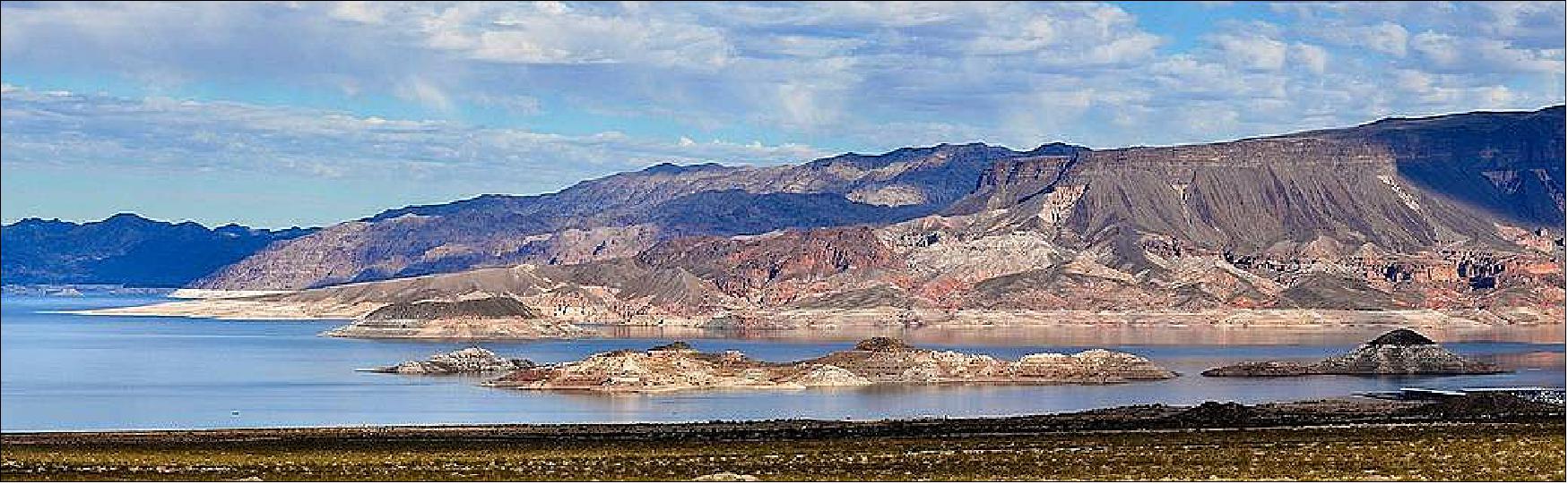
- Scientists used these height measurements to study 227,386 water bodies over 22 months and discovered that, from season to season, the water level in Earth’s lakes and ponds fluctuates on average by about 8.6 inches (0.22 m). At the same time, the water level of human-managed reservoirs fluctuate on average by nearly quadruple that amount – about 34 inches (0.86 m).
- While natural lakes and ponds outnumber human-managed reservoirs by more than 24 to 1 in their study, scientists calculated that reservoirs made up 57% of the total global variability of water storage.
- “Understanding that variability and finding patterns in water management really shows how much we are altering the global hydrological cycle,” said Sarah Cooley, a remote sensing hydrologist at Stanford University in California, who led the research. “The impact of humans on water storage is much higher than we were anticipating.”
- In natural lakes and ponds, water levels typically vary with the seasons, filling up during rainy periods and draining when it’s hot and dry. In reservoirs, however, managers influence that variation – often storing more water during rainy seasons and diverting it when it’s dry, which can exaggerate the natural seasonal variation, Cooley said.
- Cooley and her colleagues found regional patterns as well – reservoirs vary the most in the Middle East, southern Africa, and the western United States, while the natural variation in lakes and ponds is more pronounced in tropical areas.
- The results set the stage for future investigations into how the relationship between human activity and climate alters the availability of freshwater. As growing populations place more demands on freshwater, and climate change alters the way water moves through the hydrological cycle, studies like this can illuminate how water is being managed, Cooley said.
- “This kind of dataset will be so valuable for seeing how human management of water is changing in the future, and what areas are experiencing the greatest change, or experiencing threats to their water storage,” Cooley said. “This study provides us with a really valuable baseline of how humans are modulating the water cycle at the global scale.”
- The researchers’ methods relied on a second satellite mission, as well – Landsat, the decades-long mission jointly overseen by NASA and the U.S. Geological Survey. The team used Landsat-derived, two-dimensional maps of bodies of water and their sizes, providing them with a comprehensive database of the world’s lakes, ponds, and reservoirs. Then, ICESat-2 added the third dimension – height of the water level, with an uncertainty of roughly 4 inches (10 cm). When those measurements are averaged over thousands of lakes and reservoirs, the uncertainty drops even more.
- Although ICESat-2’s mission focuses on the frozen water of Earth’s cryosphere, creating data products of non-frozen water heights was also part of the original plan, according to Tom Neumann, ICESat-2 project scientist at NASA’s Goddard Space Flight Center in Greenbelt, Maryland. Now, with the satellite in orbit, scientists are detecting more smaller lakes and reservoirs than previously anticipated – in this study they detected ponds half the size of the Lincoln Memorial Reflecting Pool.
- “We’re now able to measure all of these lakes and reservoirs with the same ‘ruler,’ over and over again,” Neumann said. “It’s a great example of another science application that these height measurements enable. It’s incredibly exciting to see what questions people are able to investigate with these datasets.”
• December 9, 2020: For a satellite with ice in its name, and measuring ice as its mission, NASA’s ICESat-2 is also getting a lot of attention from scientists who have warmer subjects in mind. At this month’s Fall Meeting of the American Geophysical Union (AGU), researchers are highlighting how the Ice, Cloud and land Elevation Satellite 2 is helping to understand aspects of our home planet far beyond what it was intended to do. 41)
- When ICESat-2 sent back its first measurements on the heights of Earth’s surface in early 2019 the ICESat-2 science team lead, Lori Magruder of the University of Texas, recalls her colleague and fellow science team member Amy Neuenschwander banging on their shared office wall for her to come look at one of the first data sets: A profile of the Mexico coastline showed mountains and trees as expected, but then also continued to the ocean, where both waves at the surface as well as the seafloor below were easily distinguishable. Around the same time, Helen Fricker of Scripps Institution of Oceanography zeroed in on her favorite swath of Antarctic ice – the Amery Ice Shelf – not to look at the height of the frozen ice itself, but to see if meltwater pooling on the surface of the ice shelf was visible from space (it was).
- “It’s amazing what you can see with this data, and it just keeps sparking people's curiosity,” Magruder said.
- Before its September 2018 launch, the ICESat-2 mission team was focused on making sure the satellite met its science requirements, said Tom Neumann, the mission’s project scientist at NASA’s Goddard Space Flight Center in Greenbelt, Maryland. And it has, by precisely measuring the height of the ice sheets at Earth’s poles, of sea ice floes above the ocean waters, and of forest canopies.
- The satellite’s continuous coverage around the globe, with height measurements of Earth’s surface taken every 2.3 feet (70 cm) along its ground path, has made ICESat-2 datasets appealing to those studying rivers, coastal regions, forests and more, he said.
- “After two years, we have a lot of data over a lot of places, including some latitudes where other satellites don’t cover,” Neumann said. “This gives researchers a wealth of information to use in any number of creative ways.”
Water on ice
- During the Antarctic summer, networks of rivers and ponds appear on some ice shelves and glaciers at the edge of the continent. To estimate how much ice has melted and how much water has filled these ponds, scientists generally turn to satellite images. They infer depth based on the color of the ponds – darker blue means deeper water, Fricker said. ICESat-2’s laser instrument, however, can directly measure both the height of the top of the melt pond and of the ice below.
- Fricker and her colleagues compared the results using ICESat-2 data with results from just images. In a new study presented at the AGU meeting, they found that the imagery-only methods underestimated the depth of the melt ponds by 30% to 70%. Now, the team is working on ways to incorporate the new depth data with the imagery data. “The strength is in combining the two,” she said.
- Researchers are also using ICESat-2 to investigate the meltwater that pools on floes of Arctic sea ice – which impact how much heat from the Sun is absorbed by the planet. These ponds can be as big as Olympic-sized swimming pools, or bigger, and about 2.5 feet (80 cm) deep. Traditionally, the size of these melt ponds has been estimated based on relationships between area and depth from fieldwork done in 1998, said Sinead Farrell, an ice scientist at the University of Maryland, College Park.
- “A lot has changed in the Arctic since then – we’ve lost a lot of the thicker, older ice, and so we want to see if those observations made in the ‘90s are still representative today,” Farrell said. With the precise measurements of ICESat-2, which show ridges, cracks and ponds on the sea ice, scientists can research that question and others.
- One of Farrell’s graduate students, Ellen Buckley, also of the University of Maryland, is presenting work at the AGU meeting that describes ways to automatically detect melt ponds on sea ice in the ICESat-2 datasets, and track how they change throughout the summer season. This information could be used to help improve the sea ice forecasts used by ships navigating the Arctic.
Water on Land
- In the mountainous regions of Asia, it can be difficult to measure how much water is flowing down rivers, but it’s key for forecasting water availability as well as flood potential. Heidi Ranndal, a scientist with the Technical University of Denmark in Copenhagen, is using ICESat-2 to improve the measurements that she gets with radar satellites. She’s able to acquire thousands of useful height measurements of a river like the Yangtze from ICESat-2.
- “I was looking at an ICESat-2 track crossing the Yangtze River, and I could actually see the outline of a ship,” Ranndal said. “That was very impressive, since usually I would get just a few data points, which makes it harder to determine the height.”
- Radar satellite data, like that from the European Space Agency's CryoSat-2 or Sentinel-3, has its strengths though – those satellites measure a given area more frequently than ICESat-2 does, and also take measurements through clouds, which ICESat-2 cannot do. So she’s combining the two types of data to improve river flow estimates, and presenting the results at the AGU meeting.
Land under Water
- With ICESat-2’s ability to measure both the surface of water and the seafloor below it – up to 140 feet (43 meters) in optimal conditions – researchers are also using the satellite to investigate coastal ecosystems.
- The bathymetry of the seafloor is generally well-characterized at a global scale, but there’s a gap in knowledge about the shallow waters between the coastline and the open ocean where existing data does not contain enough detail, said Nathan Thomas, a scientist at NASA Goddard. It can be cost-prohibitive, or even dangerous, to measure these areas by ship, so he is working to combine ICESat-2 measurements with existing satellite datasets to better map coral reefs, sea grasses, tidal flats and other aquatic ecosystems.
- Thomas is also using ICESat-2 to measure mangrove forests from the tops of the trees, to the base of their roots – a tricky task given that the roots are sometimes submerged under water. If he and his colleagues can measure the full height of these trees, however, while compensating for the tides, they can calculate the stores of biomass and carbon held in these forests, and add those to the global ICESat-2 biomass inventory.
- Focusing on that same gap between land and open oceans, Brett Buzzanga of Old Dominion University in Norfolk, Virginia, is investigating how well ICESat-2 can measure sea level rise in coastal regions.
- “ICESat-2 can detect sea level changes at a high spatial resolution, and so can measure these coastal regions – it really complements other satellites and methods we use to measure sea level rise,” he said.
- He’s also presenting data at AGU that shows what appears to be a tsunami that ICESat-2 passed over at just the right time. But he’s mostly interested in the small features of the ocean processes that are hard to measure with other remote sensing tools.
- Magruder is presenting research at the AGU meeting that examines how to use ICESat-2 to improve nearshore bathymetry maps – and said she’s excited to see what other uses people come up with for the satellite’s data.
- “It’s almost like a snowball effect, with someone saying if they can map mangroves, maybe I can do coral reefs, or maybe even ocean phytoplankton,” she said. “It’s been really fun, and everyone’s so energetic about the data and the mission.”
• November 9, 2020: Just like forests can grow and shrink over time, so do glaciers, ice shelves, and ice sheets. Sometimes, ice grows through snow accumulation. Other times, it loses mass from melting or from calving icebergs. With modern satellites, scientists can measure and monitor these gains and losses with ever-increasing precision. 42)
- One key measurement for assessing the health of these frozen reservoirs is ice height, which scientists use to calculate mass changes over time. Researchers combine ice height measurements with other observations to determine the thickness and volume of a piece of ice, which is then converted into mass.
- In recent decades, Earth’s ice-covered regions have been losing more mass than they are gaining. Rising global temperatures are melting glaciers and ice sheets, reducing their thickness, length, and mass. The water from that melted ice flows into the ocean and adds to its volume: Scientists estimate that every 360 gigatons of added melt water raises global sea level by one millimeter. While melting ice is not the only contributor to sea level rise, satellite records since the 1990s show that it has been the largest contributor.
- Scientists can use radar and laser altimeters to measure changes to ice elevation. These remote sensing instruments operate by sending radio or laser light pulses toward Earth’s surface and recording the reflections as they bounce back. By measuring the time between the outgoing and returning signal, and knowing the precise altitude of the satellite above ground, scientists can calculate the elevation of the ice surface. Then by comparing multiple altimeter passes over months and years, they can derive surface changes over time.
- Although radar and laser altimeters use similar methodology, the two operate at different frequencies and return different information. Radar altimeters use microwave frequencies that illuminate large swaths on the ice sheets (for instance, a 1700-meter diameter). The instruments can “see” the surface in all atmospheric conditions, regardless of clouds, and the signals can penetrate snow to see ice layers. Lasers use shorter wavelengths that are focused into very narrow beams; they observe smaller patches of the surface. (ICESat-2, for instance, has a footprint with a 14-meter diameter.) Lasers cannot penetrate thick clouds, and their signals reflect off the top of the snow layer.
- The two types of measurements are complementary. Radars can observe more ice area with greater frequency, but less precision. Laser altimeters can return more precise data about the ice surface, particularly over steeply sloping areas, but it observes the same swaths less often.
- In 2003, NASA launched the first Earth-observing laser altimeter aboard the Ice, Cloud and land Elevation Satellite (ICESat), which was also the first altimetry mission specifically designed to observe ice. ICESat operated until 2010, and NASA launched a more advanced ICESat-2 in 2018. While the first generation satellite carried three lasers that fired 40 pulses of infrared light per second and took measurements every 170 m (560 feet), the successor carries two green lasers that fire 10,000 pulses per second and collect data every 70 cm (30 inches). ICESat-2 gathers enough data to estimate the annual height change of the Greenland and Antarctic Ice Sheets to within 4 mm (0.2 inches).
- Since July 2020, ESA’s CryoSat-2 and NASA’s ICESat-2 have been flying in orbits that periodically overlap in the Arctic in order to enable simultaneous radar and laser observations. Those synchronized overpasses will allow scientists to make better measurements of sea ice thickness.
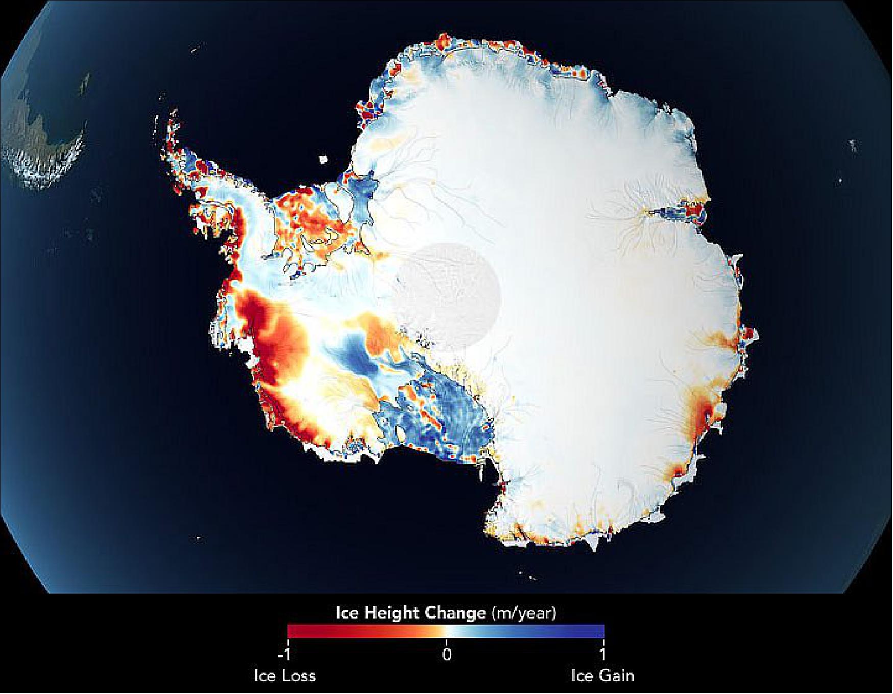
- Mass losses in Greenland exceeded those in Antarctica during those 16 years. Researchers found that Greenland lost an average of 200 gigatons of ice per year, much of it from coastal glaciers. Analyzing various datasets, the scientists found that the main driver of loss in Greenland was surface melting due to ever-warmer summer temperatures. Warmer ocean water also eroded the glaciers at their fronts in some basins.
- Antarctica’s ice sheet, which is about eight times larger than Greenland’s, has been losing around 118 gigatons of ice per year across the continent. Further analysis showed that warmer ocean temperatures caused most of the West Antarctic ice loss. Significant snow and ice accumulation in parts of East Antarctica offset some of those losses.
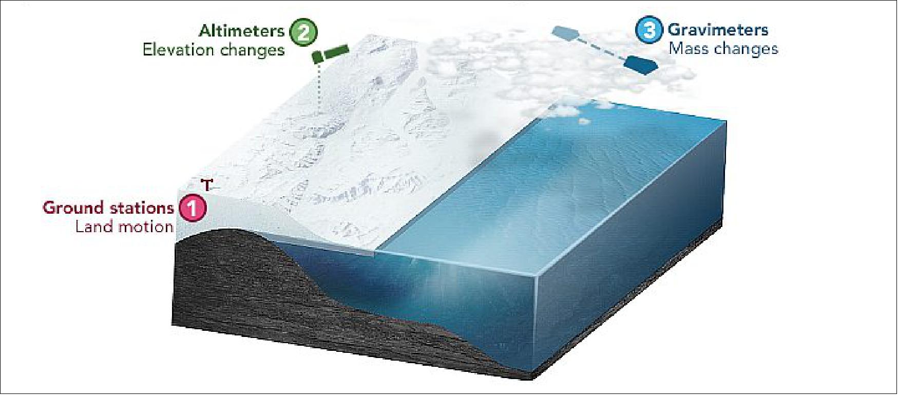
- Ice scientists are currently working to build better ice mass balance models by combining observations from ICESat and ICESat-2 with those from the Gravity Recovery and Climate Experiment (GRACE) and GRACE-Follow On satellites. Another effort called the Ice Sheet Mass Balance Inter-comparison Exercise (IMBIE) combines data from 13 NASA and ESA missions to create mass change models. Scientists also use ice height in models of how ice sheets may change in the future, such as in the Ice Sheet Model Intercomparison Project (ISMIP6) that brings together ice sheet modeling groups around the world.
- Find more stories about our changing oceans and coasts in Earth Observatory’s sea level rise collection. Explore other stories of sea level by our NASA colleagues in Rising Waters.
- Looking for data related to sea level rise? The Sea Level Change Data Pathfinder on NASA’s Earthdata site highlights tools used by researchers to study ice sheet altimetry, including ICESat Global Antarctic and Greenland Ice Sheet Altimetry Data, ICESat-2 Land Ice Height, GRACE and GRACE-FO Greenland Ice Mass Anomalies, and Antarctic Ice Mass Anomalies.
• October 27, 2020: TCarta Marine of Denver, CO, a global provider of hydrospatial products, has announced development of new Machine Learning-based bathymetric mapping technologies - including creation of two software packages and commercial application of NASA's ICESat-2 satellite - with funding from the National Science Foundation (NSF). 43)
- "The NSF grant has brought value to the bathymetric mapping arena in many ways," said TCarta President Kyle Goodrich. "We have applied the newly developed satellite-derived bathymetric (SDB) mapping techniques in numerous commercial and government projects worldwide."
- The commercial bathymetric mapping projects relate to oil spill management, oil and gas exploration and production, coastal infrastructure engineering, environmental monitoring, and geospatial intelligence (GEOINT) activities. Customers include private-sector organizations as well as numerous international government agencies.
- As TCarta begins the second year of its NSF Phase II grant, the company announced the release of two bathymetric software products developed through the program:
a) Multispectral Bathymetric Tool for Esri ArcPro - A toolbox within the popular Esri GIS software to process Satellite Derived Bathymetry data, assess accuracy, and output as .BAG files.
b) ICESat Data Extraction Software - A tool that leverages artificial intelligence algorithms to automatically extract seafloor depth measurements from ICESat-2 laser data.
- In 2018, NSF awarded TCarta a Phase 1 grant to develop multi-method and integrate SDB technologies. Referred to as Project Trident, the research focused on leveraging Artificial Intelligence (AI) - machine learning and computer vision - to determine shallow-water seafloor depths in variable water conditions. The two-year Phase 2 grant focused on commercialization of these technologies was awarded in late 2019.
- "An exciting addition to Project Trident was NASA's ICESat-2 satellite data, which we incorporated into the workflow as a validation tool and algorithm training for the enhanced SDB technologies currently under development," said Goodrich. "TCarta became the first to integrate the ICESat-2 laser measurements into commercial bathymetric projects and now routinely offer these enhancements."
- Developed by NASA and the University of Texas, ICESat-2 (Ice, Cloud and land Elevation Satellite) was designed primarily for polar ice elevation and tree canopy measurements, but the green laser altimeter onboard has proved remarkably accurate at gauging seafloor depths down to 100 feet below the surface.
- By combining the ML-based SDB techniques with the ICESat-2 validation methods, TCarta developed an entirely new workflow for deriving highly accurate water depth measurements at scale from multiple high-resolution satellite images for large coastal areas. In the past year, TCarta has deployed this technique in high-profile projects:
- WV Wakashio grounding & Oil Spill – In the immediate aftermath of the Indian Ocean shipwreck off the coast of Mauritius, TCarta acquired Maxar WorldView-2 satellite imagery over the poorly charted area and applied the new ICESat-validated SDB method to map the seafloor. The bathymetric data sets were published via web mapping service and made freely available through Esri’s ArcGIS Online and Maxar’s SecureWatch platforms.
- Hurricane Dorian Response & Isaias Threat – Demonstrating the ability to scale up the SDB method to include a multitude of images, TCarta applied the technology to process over 400 Sentinel 2 satellite images over the Bahamas region from post hurricane Dorian imagery and validated with millions of ICESat-2 data points. The result was a 10-meter bathymetric map covering 130,000 km2 provided via the Esri Caribbean GeoPortal to organizations engaged in hurricane preparedness activities ahead of Hurricane Isaias.
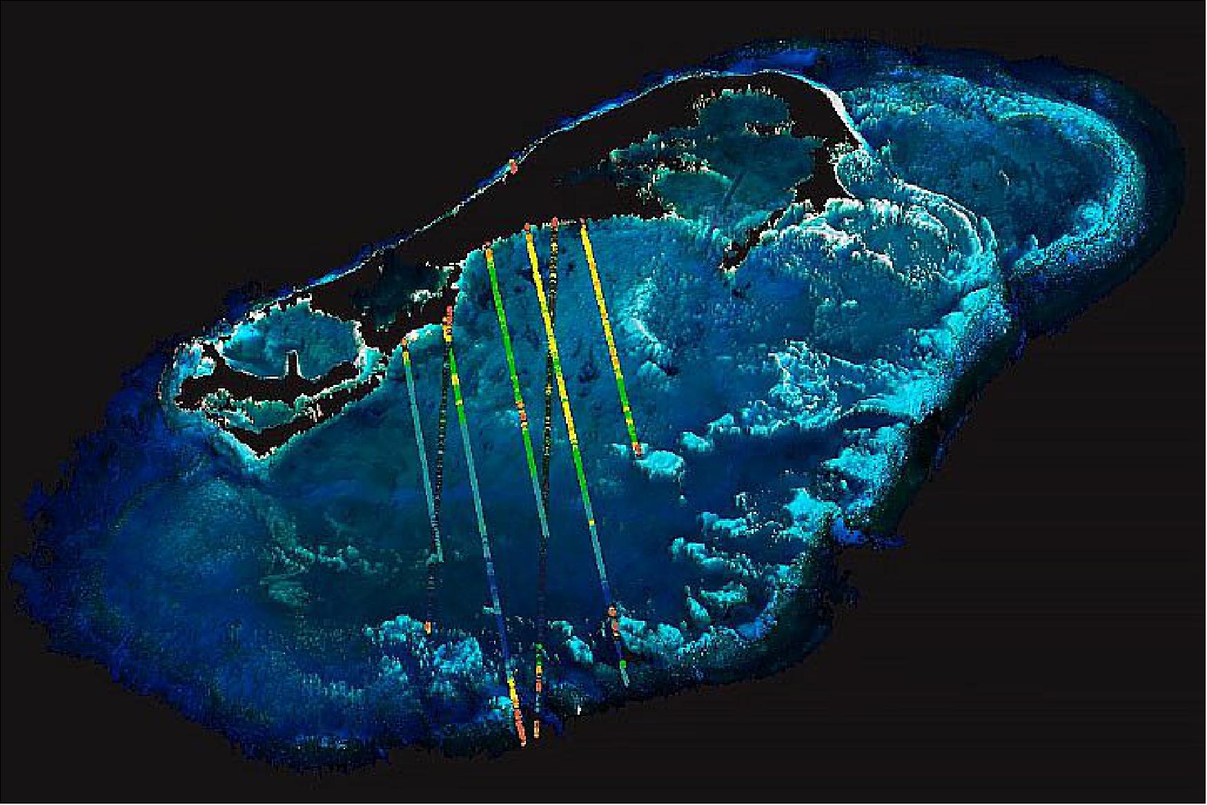
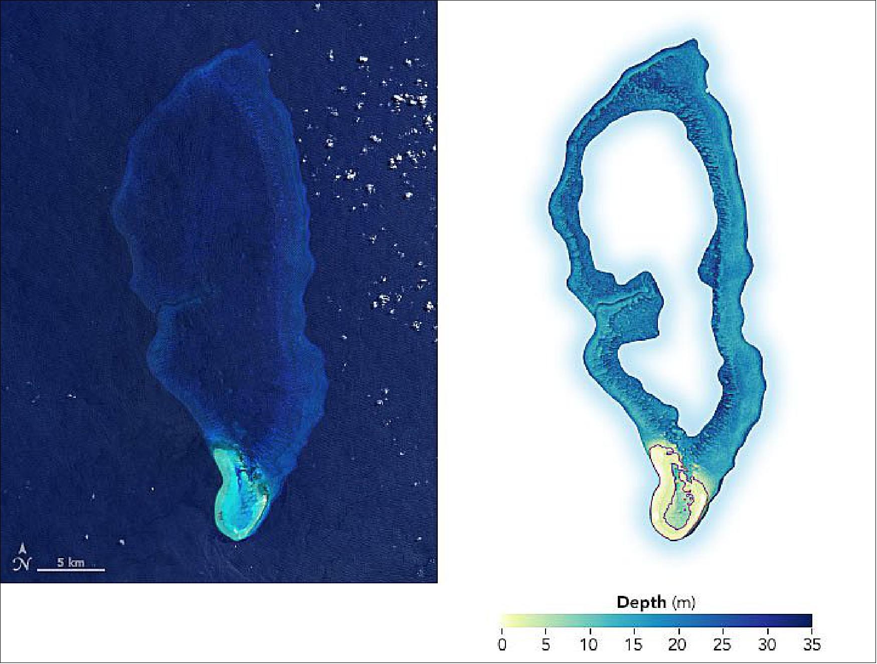
• September 29, 2020: The waters along the world’s coasts and islands are incredibly important to human activities, yet they are not always well mapped. Coastal waters are often turbulent and murky, as the sand, mud, and sediment on the bottom is constantly in motion. Unless there are regularly dredged channels, it can be difficult and dangerous for ships to travel in shallow water. Making accurate and up-to-date depth charts is time-consuming and expensive, and doing so on a global scale is a monumental task. 44)
- By combining satellite measurements with ship-based sonar data, a team of researchers is now working to fill the gaps in our seafloor maps. They are using data from NASA’s Ice, Cloud, and land Elevation Satellite 2 (ICESat-2) to accurately measure the depths (bathymetry) of shallow coastal waters, where surveying ships have historically been unable to travel due to safety, expense, or remoteness.
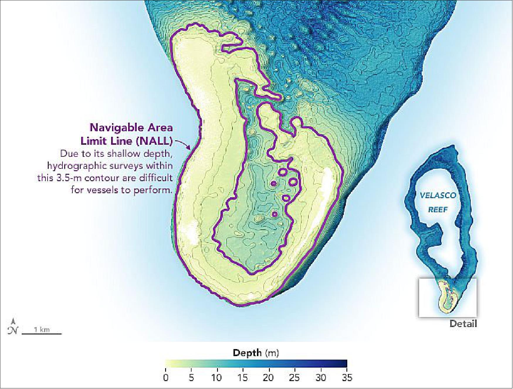
- Mapping shallow, nearshore areas can be slow and potentially dangerous. Conventional field methods may involve a surveyor standing in shallow water, taking measurements at specific intervals, while at the mercy of waves and currents. Meanwhile, boat-based sonar surveys are inefficient in shallow waters and subject to the dangers of waves, rocks, and reefs. In addition, the National Oceanic and Atmospheric Administration (NOAA) has established Navigable Area Limit Lines (NALL), which define the shoreward limit of their boat-based surveys. The NALL is set at water depths of 3.5 meters (11 feet), and NOAA advises caution to captains maneuvering in shallow areas within the NALL because they are not often mapped, if at all. Sometimes the NALL limit can extend significant distances from shore.
- These challenges result in many nearshore coastal waters being largely unmapped. The area is nicknamed “the white ribbon” because it appears as white space hugging coasts, shoals, and atolls on bathymetric maps. It essentially represents no data.
- “The near-coastal area from 0 to 10 meters in depth is notoriously hard to map because a lot of the acoustic sensors that are used in bathymetry do not capture the shallower depths accurately,” said Magruder. “ Near-shore measurements provide a window into the coastal dynamics and processes that are really important.”
- The satellite’s main instrument is the ATLAS altimeter, which sends 10,000 laser pulses per second toward Earth’s surface and detects the photons that return in order to determine the height of landmasses and features on it (such as ice sheets, forests, and glaciers). It turns out that ICESat-2’s laser pulses can also penetrate the water column in shallow areas and return measurements from the seafloor.
- The main mission of ICESat-2 is to map sea ice thickness and ice sheet elevation, as well as the height and density of temperate and tropical forests. Scientists and engineers thought it might be possible to measure ocean bathymetry, but they were not sure until Adrian Borsa, a geodesist at the University of California, San Diego, noticed in 2018 that ICESAT-2 data was picking up seafloor signals around Bikini Atoll in the South Pacific.
- This finding provoked Parrish and Magruder to make a concentrated effort to use the satellite for near-shore mapping. Because it can observe across the entire globe, ICESat-2 provides broader spatial coverage than sonar-mapping ships. The satellite also collects data from the same location every 91 days, allowing for repeat mapping of areas that previously took great effort to map even once.
- Beyond Velasco Reef, researchers are using the novel dataset to map near-shore habitats off of Western Australia and around the Gilbert Islands, French Polynesia, Turks and Caicos, and the Bahamas. The methods are even being used to map the shores of Lake Tahoe, California. With a complete and continuous look at near-shore bathymetry, researchers can aid efforts to monitor endangered coral reefs and coastal mangroves, sediment transport after disaster events, carbon storage capacity, water clarity, invasive species, and several other aspects of coastal dynamics.
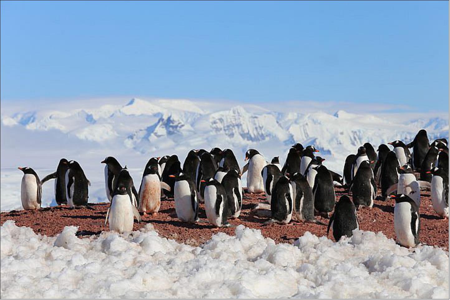
• September 24, 2020: Recent censuses of the tuxedoed inhabitants of the Antarctic Peninsula have shown intriguing differences between species. Populations of Adélie and chinstrap penguins are declining, while populations of gentoo penguins are growing. Remote sensing data are helping scientists figure out why. 45)
- “The gentoo penguin is a climate change winner, with populations moving farther south than we have ever seen them,” said Michael Wethington, a graduate student at Stony Brook University. “New colonies generally happen very rarely, but we have spotted a slew of new ones in past five to ten years.”
- Wethington thinks gentoo penguins might be taking advantage of food sources farther south along the peninsula—a move that requires sea ice conditions to be just right. Populations of krill, a staple of the penguin diet, flourish where there is ample sea ice. But suitable penguin habitat requires at least some openings in the ice where they can access the ocean to hunt and forage. And because gentoos overwinter near their summer breeding colonies, their survival each year depends on nearby “hunting holes” that stay open throughout the cold, dark austral winter.
- “To understand penguin habitat, it is important to understand what is happening with sea ice dynamics surrounding their colonies,” Wethington said. “Satellite data are enabling us to identify and better understand the locations where open water foraging habitat exist and the trends throughout the year.”
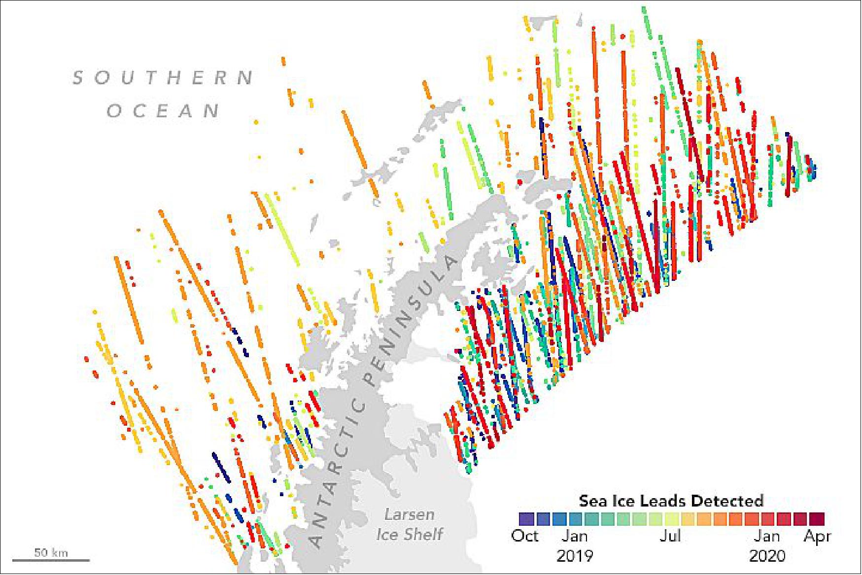
- During sunlit months, light reflected from Earth’s surface allows passive satellite sensors to collect images of sea ice and the various cracks or fractures (leads) where there is open water. But the lack of sunlight during the winter months means these sensors cannot observe these surface features, leaving scientists in the dark about penguin habitat.
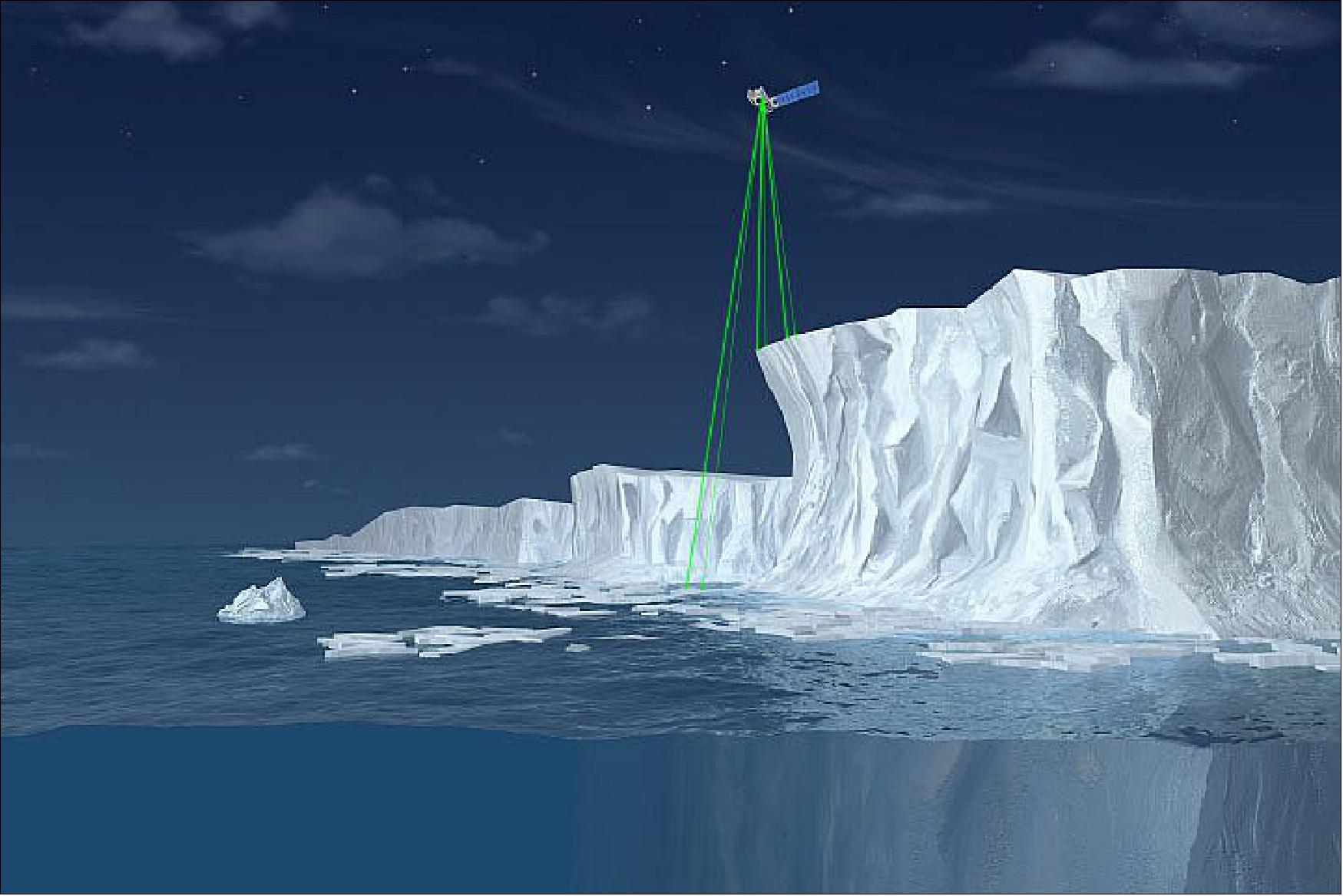
- Winter darkness is not a problem for NASA’s Ice, Cloud and land Elevation Satellite-2 (ICESat-2). The satellite carries a laser altimeter that uses pulses of light to precisely measure the height of the first substance it hits, whether that’s open water or sea ice. Open water within a lead shows up in the satellite data as a very flat surface, as opposed to the comparatively textured surface of sea ice. These data provide a high-resolution look at the location and width of leads in the sea ice.
- “This approach represents a new chapter of using active remote sensing to better understand the environmental drivers impacting populations during a time of year that has so often remained a mystery to researchers,” Wethington said.
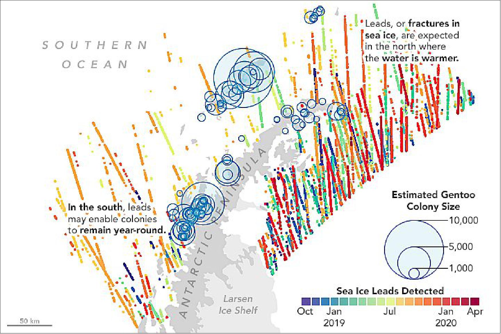
- Wethington said the next step in the investigation involves building a statistical model to investigate how lead density and proximity to penguin colonies affect population trends from year to year, as well as their importance for enabling new colonies to be established.
- “This was a really nice and unique use of ICESat-2 data,” said Nathan Kurtz, a sea ice scientist at NASA’s Goddard Space Flight Center and deputy project scientist for ICESat-2. “Studies like this weren’t part of the primary science objectives from ICESat-2, but it has been very interesting to see what new types of science can be done to understand different aspects of our planet.”
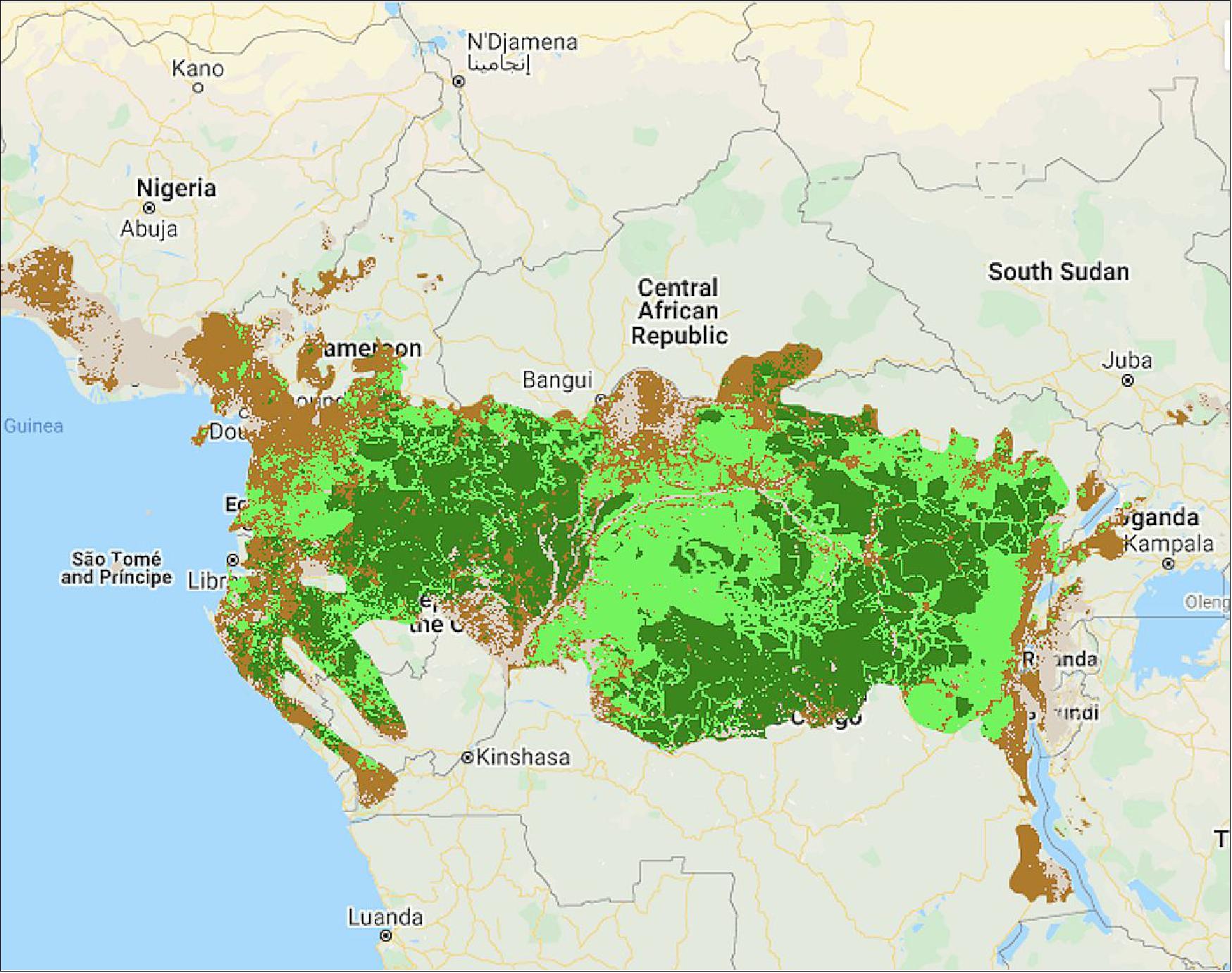
• August 25, 2020: High-resolution NASA satellite data have made it possible for scientists to develop maps showing the "quality" of tropical forests. Previous maps only focused on the size of a forest. These maps show forest quality as a single measurement, taking into account information like the height of trees, thickness of the forest canopy, and if logging, fire or a similar disturbance occurred. 46)
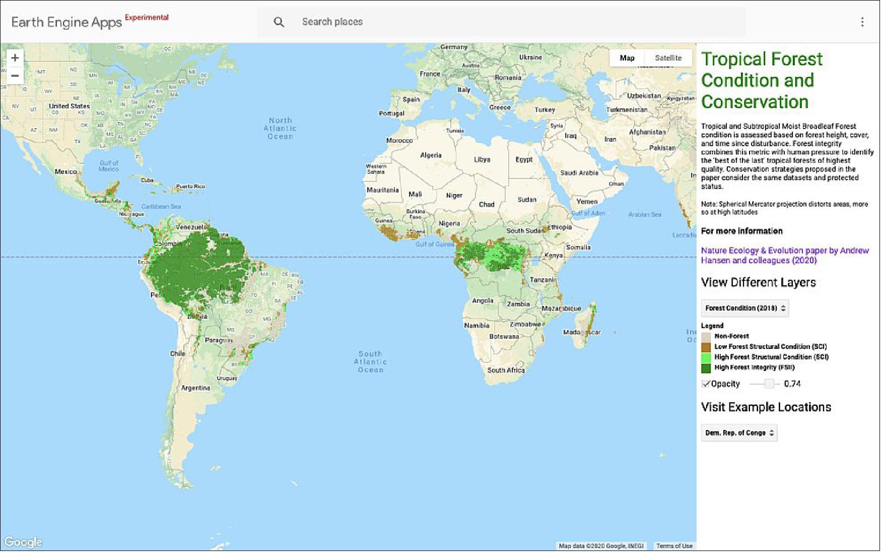
- "Now we have maps that show, not just where the forests are located, but the ecological quality of those forests," said lead author Andrew Hansen of Montana State University.
- "That's important because it allows policy makers to prioritize forests that have the highest value in terms of biodiversity, carbon storage and water yield," Hansen said.
- About half of the world's humid tropical forests could be considered of "high quality," according to the study published in the journal Nature Ecology & Evolution. The study was supported the United Nations Development Program (UNDP), the Wildlife Conservation Society and other leading research institutions. 47)
- Only 6.5% of these high-quality forests have formal protections, said Hansen. With their low levels of human pressure, large trees and thick canopy vegetation, these forests act as key habitats for many plants and animals, which fosters biodiversity. They also help stabilize the climate worldwide by absorbing carbon dioxide from the atmosphere. The paper's authors note where these high-quality forests are at risk and include a conservation framework that recommends ways to protect existing forests as well as restoring others.
- One way to restore the quality of forests is increasing the number of species that live there by strengthening protections like limiting hunting and reducing invasive species, Hansen said. "Another way is restoring forest structure," he added. "Grow taller forests with more canopy layers for example."
- Most of the high-quality forests mapped in the study are located in remote areas of the Amazon and Congo. Earth Engine: Tropical Forest Condition and Conservation
- "The key advance here was remote sensing," Hansen said, adding that Earth observations now make it possible to measure details like forest height and vegetation in far greater detail than ever before.
- "It's a globally consistent, fine-scale measurement of forest structure and allows identification of taller, older and more closed-canopy humid tropical forests," Hansen said. By combining that information with measurements of human activity, the team developed their overall index of forest quality.
• July 16, 2020: With a small nudge to a satellite’s orbit, scientists will soon have simultaneous laser and radar measurements of ice, providing new insights into Earth’s frozen regions. On July 16, the European Space Agency (ESA) begins a series of precise maneuvers that will push the orbit of its radar-carrying CryoSat-2 satellite about half a mile higher – putting it in sync with NASA’s laser-carrying ICESat-2 (Ice, Cloud and land Elevation Satellite-2). 48)
- When the maneuvers are complete later this summer, the two satellites will pass over a swath of the Arctic within a few hours of each other. That synchronous stretch, of more than 2,000 miles (3,200 kilometers) every day or so, will be key for studying sea ice, which floats on the Arctic Ocean and is moved around with currents and winds. If the satellites take measurements at different times, the two could be measuring different floes of fast-moving ice. Syncing up the satellites provides scientists with two datasets for the same ice.
- “Combining these two measurements from space will lead to a golden age,” said Tommaso Parrinello, CryoSat-2 mission manager with ESA. “It’s a small change for CryoSat-2, but will be a revolution for the science.”
- Both CryoSat-2’s radar and ICESat-2’s laser instrument, called a lidar, measure height by sending out signals and timing how long they take to reflect off Earth’s surface and return to their respective satellites. But the different signals bounce off some surfaces differently – including snow-covered sea ice. Radars like CryoSat-2’s will penetrate through the snow layer and reflect off the ice below. Laser instruments like ICESat-2’s will reflect off the top of the snow layer. The difference between the two will give scientists the depth of the snow atop sea ice.
- “If you have laser and radar together, it gives you this really exciting opportunity to measure the depth of the snow, which we’ve really never been able to do before from space,” said Rachel Tilling, a sea ice scientist at NASA’s Goddard Space Flight Center in Greenbelt, Maryland and the University of Maryland in College Park. “And with snow depth, we can get significantly more accurate measurements of sea ice thickness.”
- With better measurements of snow depth and sea ice thickness, researchers can gain insights into the complex Arctic climate system. Sea ice might just be 10 feet thick or so, but it has an outsized effect on Earth’s climate, forming a kind of a protective blanket on the Arctic Ocean, Tilling said. The snow on top reflects radiation from the Sun, keeping the ice from melting and the ocean from warming. The ice itself acts as a barrier between the atmosphere and the ocean – removing it could alter circulation patterns that reach the more temperate parts of the globe. The new information could improve climate models, as well as lead to more accurate shipping navigation forecasts, she said.
- The idea of aligning the two satellites has been floating around among the ice science community since CryoSat-2 launched in 2010, when ICESat-2 was still in the development stage, said Tom Neumann, ICESat-2 project scientist at NASA Goddard.
- “This opens up new science possibilities that weren’t possible with either mission independently, especially for sea ice science,” Neumann said. “It’s a grassroots effort, promoted by the scientists and engineers asking if there was a way we can make this happen.”
- The CryoSat-2 flight operations team took a look and after months of analyzing orbital dynamics came up with a plan. The European satellite orbits much higher and slower than the American one, so they couldn’t simply follow each other in tandem, said Ignacio Clerigo, CryoSat-2’s spacecraft operations manager. Instead, they realized they could raise the altitude of the spacecraft by just more than half a mile (900 meters), through a series of 15 precisely timed thruster burns, and then the two satellites would overlap every 19th orbit of CryoSat-2 and 20th orbit of ICESat-2. The overlaps are mostly over the Arctic; next Northern Hemisphere summer ESA might precisely alter the orbit again with another set of maneuvers to focus on the Antarctic during that region’s winter.
- “It’s a challenge, not because of the maneuvers themselves, but because of the tight schedule,” Clerigo said. “We have continuous activities for two weeks. Each step depends on the previous one and if something does not go as expected, we will need to replan quickly to reach the target orbit.”
• May 27, 2020: For the past two decades, satellites and scientists have revealed an ongoing, decades-long decline in Arctic sea ice, with implications for global ecosystems, weather, and climate. Satellites are now tracking what’s happening to the reflective, insulating layer of snow atop the ice. 49)
- The snow layer is an important component of the sea ice system, affecting how the ice grows and melts. In winter, blanket-like snow cover insulates sea ice from frigid polar air, slowing ice growth. In spring, snow cover must melt away before the ice surface can begin to melt. By summer, melt water from the snow collects in ponds atop the ice; this water absorbs heat from the Sun and can accelerate the warming and melting of the ice.
- Over the years, scientists have collected ground and airborne surveys of snow depth here and there. But they need routine, widespread measurements to detect the detailed variations in snow depth across the ice cap and how it changes during the year. Those details are now measurable, as scientists have created the first satellite-based maps of snow accumulation on Arctic sea ice.
- “This is the first time ever that we can get snow depth across the entire Arctic Ocean’s sea ice cover,” said Ron Kwok, a sea ice scientist at NASA’s Jet Propulsion Laboratory and author of a study in JGR Oceans. “The Arctic region is a desert—but what snow we do get is very important in terms of the climate and insulating sea ice.” 50)
- To produce the maps, scientists compared elevation measurements from two satellites. NASA’s Ice, Cloud and land Elevation Satellite-2 (ICESat-2) carries a laser altimeter, which uses pulses of light to precisely measure the height of the first substance it hits—whether that’s open water, bare sea ice, or snow that has accumulated on top of the ice. The European Space Agency’s CryoSat-2 satellite carries a radar altimeter; in contrast to lidar, the radio waves of radar mostly pass through snow and reflect off the top of the ice. By calculating the difference between these two measurements, scientists can estimate the depth of the snow layer on top.
- “The method is certainly the best approach to-date,” Kwok said. “With ICESat-2 and CryoSat-2, we are able to obtain a time-variable estimate of the snow depth from observations, without resorting to models.”
- With additional years of observations, maps like these could help scientists assess how climate change affects precipitation and the accumulation of snow. The challenge, Kwok notes, is that the measurement relies on having both satellites in orbit at the same time. ICESat-2 is newer, having launched in 2018, while CryoSat-2 has already been in orbit for a decade.
- “If we lose CryoSat-2, then we are back to doing this with ICESat-2 alone,” Kwok said. “The hope is that we’ll be able to have a least a few years to make progress toward improving models.”
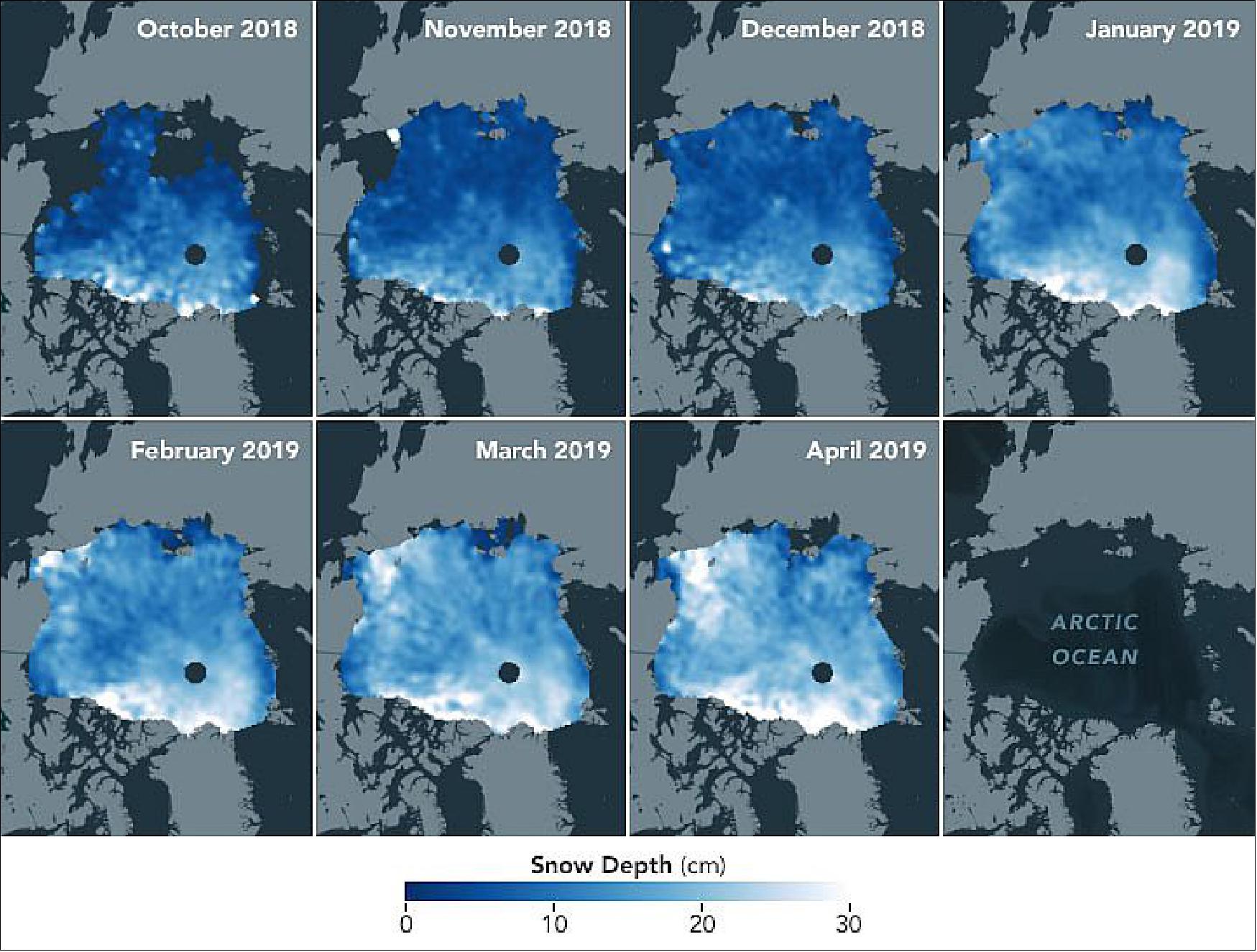
• May 14, 2020: Arctic sea ice helps keep Earth cool, as its bright surface reflects the Sun’s energy back into space. Each year scientists use multiple satellites and data sets to track how much of the Arctic Ocean is covered in sea ice, but its thickness is harder to gauge. Initial results from NASA’s new Ice Cloud and land Elevation Satellite-2 (ICESat-2) suggest that the sea ice has thinned by as much as 20% since the end of the first ICESat mission (2003-2009), contrary to existing studies that find sea ice thickness has remained relatively constant in the last decade. 51)
- ICESat-2 has a laser altimeter, which uses pulses of light to precisely measure height down to about an inch. Each second, the instrument sends out 10,000 pulses of light that bounce off the surface of Earth and return to the satellite and records the length of time it takes to make that round trip. The light reflects off the first substance it hits, whether that’s open water, bare sea ice or snow that has accumulated on top of the ice, so scientists use a combination of ICESat-2 measurements and other data to calculate sea ice thickness.
- By comparing ICESat-2 data with measurements from another satellite, researchers have also created the first satellite-based maps of the amount of snow that has accumulated on top of Arctic sea ice, tracking this insulating material.
- “The Arctic sea ice pack has changed dramatically since monitoring from satellites began more than four decades ago,” said Nathan Kurtz, ICESat-2 deputy project scientist at NASA’s Goddard Space Flight Center in Greenbelt, Maryland. “The extraordinary accuracy and year-round measurement capability of ICESat-2 provides an exciting new tool to allow us to better understand the mechanisms leading to these changes, and what this means for the future.”
- Arctic sea ice thickness dropped drastically in the first decade of the 21st Century, as measured by the first ICESat mission from 2003 to 2009 and other methods. The European Space Agency’s CryoSat-2, launched in 2010, has measured a relatively consistent thickness in Arctic sea ice since then. With the launch of ICESat-2 in 2018, researchers looked to this new way of measuring sea ice thickness to advance the study of this data record.
- “We can’t get thickness just from ICESat-2 itself, but we can use other data to derive the measurement,” said Petty. For example, the researchers subtract out the height of snow on top of the sea ice by using computer models that estimate snowfall. “The first results were very encouraging.”
- In their study, published recently in the Journal of Geophysical Research: Oceans, Petty and his colleagues generated maps of Arctic sea ice thickness from October 2018 to April 2019 and saw the ice thickening through the winter as expected. 52)
- Overall, however, calculations using ICESat-2 found that the ice was thinner during that time period than what researchers have found using CryoSat-2 data. Petty’s group also found that small but significant 20% decline in sea ice thickness by comparing February/March 2019 ICESat-2 measurements with those calculated using ICESat in February/March 2008 – a decline that the CryoSat-2 researchers don’t see in their data.
- These are two very different approaches to measuring sea ice, Petty said, each with its own limitations and benefits. CryoSat-2 carries a radar to measure height, as opposed to ICESat-2’s lidar, and radar mostly passes through snow to measure the top of the ice. Radar measurements like the ones from CryoSat-2 could be thrown off by seawater flooding the ice, he noted. In addition, ICESat-2 is still a young mission and the computer algorithms are still being refined, he said, which could ultimately change the thickness findings.
- “I think we’re going to learn a lot from having these two approaches to measuring ice thickness. They might be giving us an upper and lower bound on the sea ice thickness, and the right answer is probably somewhere in between,” Petty said. “There are reasons why ICESat-2 estimates could be low, and reasons why CryoSat-2 could be high, and we need to do more work to understand and bring these measurements in line with each other.”
- With ICESat-2 and CryoSat-2 using two different methods to measure ice thickness – one measuring the top of the snow, the other the boundary between the bottom of the snow layer and the top of the ice layer – but researchers realized they could combine the two to calculate the snow depth.
- “This is the first time ever that we can get snow depth across the entire Arctic Ocean’s sea ice cover,” said Ron Kwok, a sea ice scientist at NASA’s Jet Propulsion Laboratory in Southern California and author of another study in JGR Oceans. “The Arctic region is a desert – but what snow we do get is very important in terms of the climate and insulating sea ice.” 53)
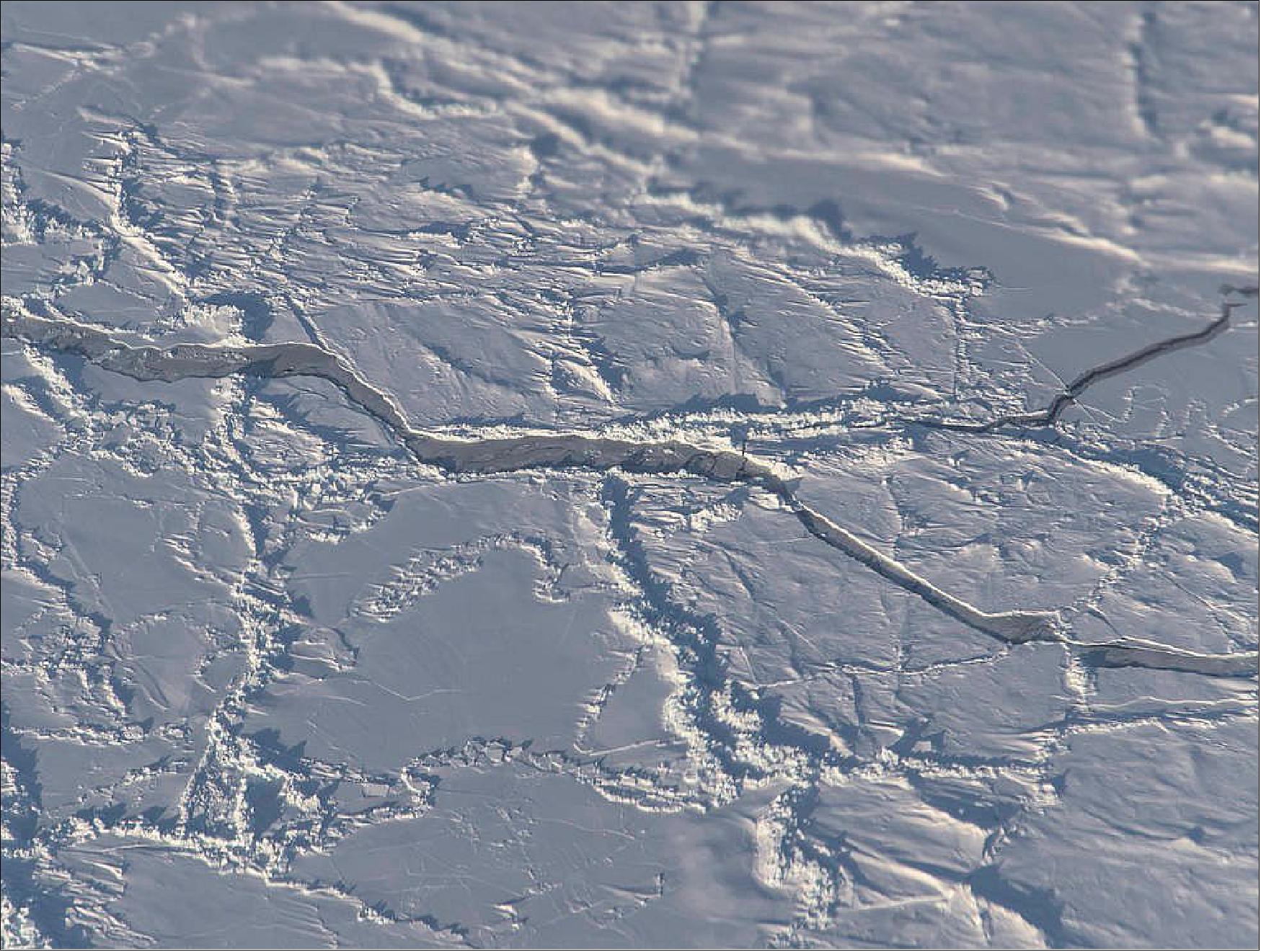
- The study found that snow starts building up slowly in October, when newly formed ice has an average of about 2 inches (5 cm) of snow on it and multiyear ice has an average of 5.5 inches (14 cm) of snow. Snowfall picks up later in the winter in December and January and reaches its maximum depth in April, when the relatively new ice has an average of 6.7 inches (17 cm) and the older ice has an average of 10.6 inches (27 cm) of snow.
- When the snow melts in the spring, it can pool up on the sea ice – those melt ponds absorb heat from the Sun and can warm up the ice faster, just one of the impacts of snow on ice.
• April 30, 2020: Using the most advanced Earth-observing laser instrument NASA has ever flown in space, scientists have made precise, detailed measurements of how the elevation of the Greenland and Antarctic ice sheets have changed over 16 years. 54)
- The results provide insights into how the polar ice sheets are changing, demonstrating definitively that small gains of ice in East Antarctica are dwarfed by massive losses in West Antarctica. The scientists found the net loss of ice from Antarctica, along with Greenland's shrinking ice sheet, has been responsible for 0.55 inches (14 mm) of sea level rise between 2003 and 2019 - slightly less than a third of the total amount of sea level rise observed in the world's oceans.
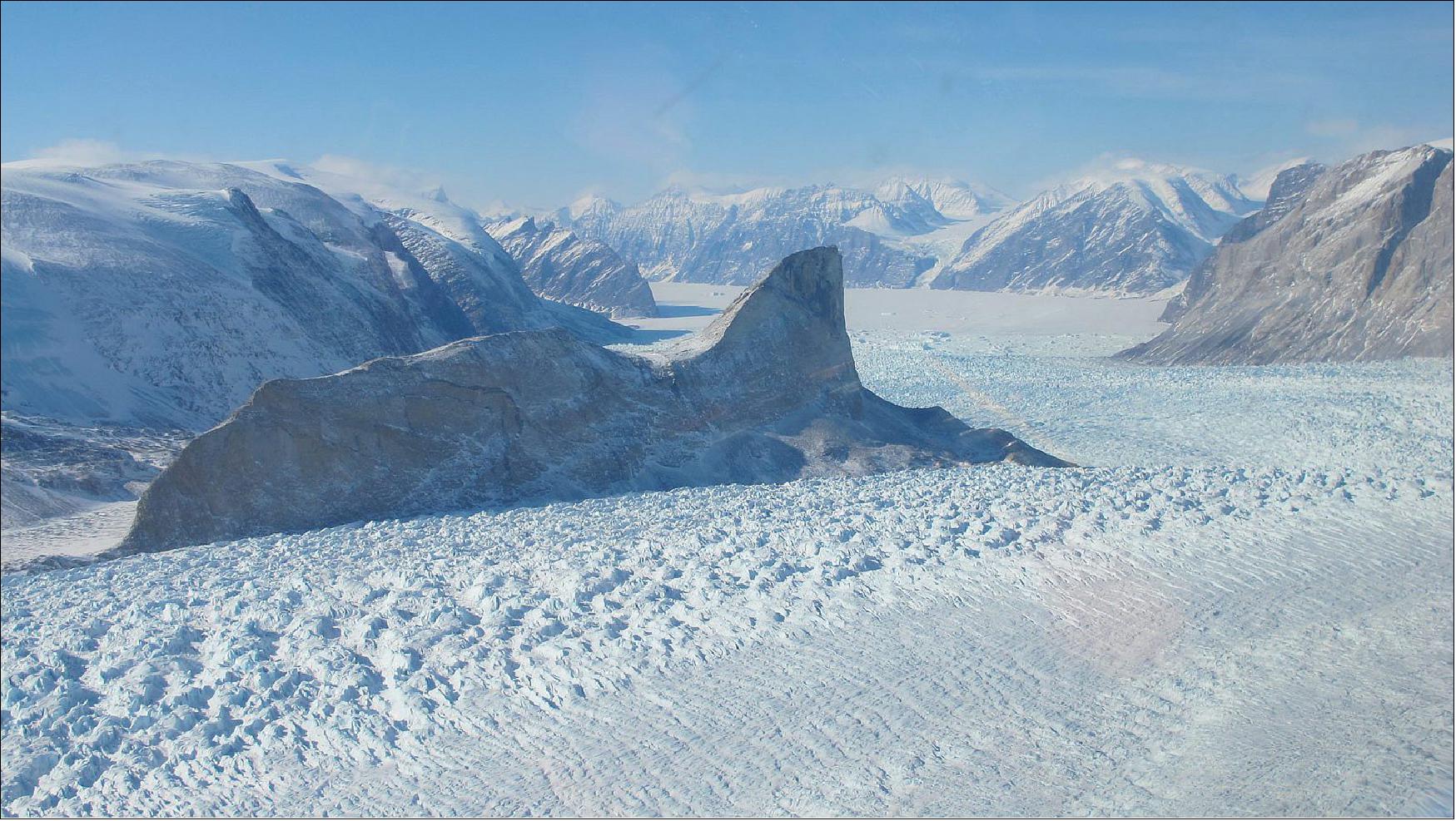
- The findings come from NASA's ICESat-2 (Ice, Cloud and land Elevation Satellite- 2), which launched in 2018 to make detailed global elevation measurements, including over Earth's frozen regions. By comparing the recent data with measurements taken by the original ICESat from 2003 to 2009, researchers have generated a comprehensive portrait of the complexities of ice sheet change and insights about the future of Greenland and Antarctica.
- The study found that Greenland's ice sheet lost an average of 200 gigatons (200 x 109 tons, corresponding to 200 km3) of ice per year, and Antarctica's ice sheet lost an average of 118 gigatons of ice per year. 55)
- "If you watch a glacier or ice sheet for a month, or a year, you're not going to learn much about what the climate is doing to it," said Ben Smith, a glaciologist at the University of Washington and lead author of the new paper, published online in Science on April 30. "We now have a 16-year span between ICESat and ICESat-2 and can be much more confident that the changes we're seeing in the ice have to do with the long-term changes in the climate."
- ICESat-2's instrument is a laser altimeter, which sends 10,000 pulses of light a second down to Earth's surface and times how long it takes to return to the satellite - to within a billionth of a second. The instrument's pulse rate allows for a dense map of measurement over the ice sheet; its high precision allows scientists to determine how much an ice sheet changes over a year to within an inch.
- The researchers took tracks of earlier ICESat measurements and overlaid the tracks of ICESat-2 measurements from 2019, and took data from the tens of millions of sites where the two data sets intersected. That gave them the elevation change, but to get to how much ice has been lost, the researchers developed a new model to convert volume change to mass change. The model calculated densities across the ice sheets to allow the total mass loss to be calculated.
- "These first results looking at land ice confirm the consensus from other research groups, but they also let us look at the details of change in individual glaciers and ice shelves at the same time," said Tom Neumann, ICESat-2 project scientist at NASA Goddard.
- In Antarctica, for example, the detailed measurements showed that the ice sheet is getting thicker in parts of the continent's interior as a result of increased snowfall, according to the study. But the loss of ice from the continent's margins, especially in West Antarctica and the Antarctic Peninsula, far outweighs any gains in the interior. In those places, the loss is due to warming from the ocean.
- In Greenland, there was a significant amount of thinning of coastal glaciers, Smith said. The Kangerdulgssuaq and Jakobshavn glaciers, for example, have lost 14 to 20 feet (4 to 6 meters) of elevation per year - the glacial basins have lost 16 gigatons per year and 22 gigatons per year, respectively. Warmer summer temperatures have melted ice from the surface of the glaciers and ice sheets, and in some basins the warmer ocean water erodes away the ice at their fronts.
- "The new analysis reveals the ice sheets' response to changes in climate with unprecedented detail, revealing clues as to why and how the ice sheets are reacting the way they are," said Alex Gardner, a glaciologist at NASA's Jet Propulsion Laboratory in Southern California, and co-author on the Science paper.
- The study also examined ice shelves - the floating masses of ice at the downstream end of glaciers. These ice shelves, which rise and fall with the tides, can be difficult to measure, said Helen Amanda Fricker, a glaciologist at Scripps Institution of Oceanography at the University of California San Diego, and co-author on the Science paper. Some of them have rough surfaces, with crevasses and ridges, but the precision and high resolution of ICESat-2 allows researchers to measure overall changes.
- This is one of the first times that researchers have used laser altimetry to measure loss of the floating ice shelves around Antarctica simultaneously with loss of the continent's ice sheet.
- The researchers found ice shelves are losing mass in West Antarctica, where many of the continent's fastest-moving glaciers are located as well. Patterns of thinning over the ice shelves in West Antarctica show that Thwaites and Crosson ice shelves have thinned the most, an average of about 16 feet (5 meters) and 10 feet (3 meters) of ice per year, respectively.
- Ice that melts from ice shelves doesn't raise sea levels, since it's already floating - just like an ice cube in a full cup of water doesn't overflow the glass when it melts. But the ice shelves do provide stability for the glaciers and ice sheets behind them.
- "It's like an architectural buttress that holds up a cathedral," Fricker said. "The ice shelves hold the ice sheet up. If you take away the ice shelves, or even if you thin them, you're reducing that buttressing force, so the grounded ice can flow faster."
• December 13, 2019: For eleven years from 2009 through 2019, the planes of NASA’s Operation IceBridge flew above the Arctic, Antarctic and Alaska, gathering data on the height, depth, thickness, flow and change of sea ice, glaciers and ice sheets. 56)
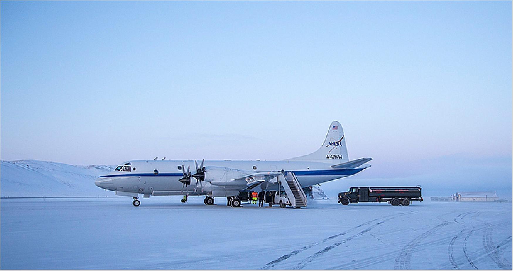
- Designed to collect data during the years between NASA’s two Ice, Cloud, and land Elevation Satellites, ICESat and ICESat-2, IceBridge made its final polar flight in November 2019, one year after ICESat-2’s successful launch. — As the team and planes move on to their next assignments, the scientists and engineers reflected on a decade of IceBridge’s most significant accomplishments.
2009: IceBridge’s Launch and First Flights
- NASA’s first Ice, Cloud, and land Elevation Satellite (ICESat) monitored ice, clouds, atmospheric particles and vegetation globally beginning in 2003. As ICESat neared the end of its life, NASA made plans to keep measuring ice elevation with aircraft until ICESat-2’s launch. ICESat finished its service in August 2009, and IceBridge took over land and sea ice measurements for the next decade.
- The number and models of IceBridge aircraft changed from year to year, and they carried more than a dozen instruments, from elevation-mapping lasers and ice-penetrating radars, to optical and infrared cameras, to gravimeters and magnetometers that reveal information about the bedrock under the ice. Beyond simply bridging the altimetry gap, the mission’s comprehensive suite of instruments allowed it to document fast and slow changes to the ice sheets, understand the geophysical causes of those changes, track yearly fluctuations in sea ice thickness and improve computing and modeling tools for research.
- Before IceBridge, NASA was annually monitoring vulnerable areas of the Greenland Ice Sheet via the Arctic Ice Mapping Project (AIM). But IceBridge far surpassed previous campaigns in size and scope, with annual surveys of both poles, more instruments and a longer timeframe that allowed it to track changes across and even within years.
- One of IceBridge’s first important contributions was mapping hundreds of miles of grounding lines in both Antarctica and Greenland. Grounding lines are where a glacier’s bottom loses contact with the bedrock and begins floating on seawater. A grounding line that is higher than rock that the ice behind it is resting on increases the possibility of future unstable retreat.
- “Before IceBridge, we had a lot of glaciers where we didn’t have information on their grounding lines, which made it challenging to model them and develop reliable projections of sea level rise,” said Michael Studinger, team lead for the Airborne Topographic Mapper (ATM) instrument and IceBridge’s project scientist from 2010 to 2015.
- “Before IceBridge, we had a lot of glaciers where we didn’t have information on their grounding lines, which made it challenging to model them and develop reliable projections of sea level rise,” said Michael Studinger, team lead for the Airborne Topographic Mapper (ATM) instrument and IceBridge’s project scientist from 2010 to 2015.
• November 1, 2019: In the opening chapter of Dracula, Bram Stoker described the Transylvanian landscape as “an endless perspective of jagged rock and pointed crags...” It was one of the few kernels of reality in an otherwise fantastic tale about the world’s most famous vampire. 57)
- The setting for Dracula is the Southern Carpathian Mountains, also called the Transylvanian Alps. The average elevation in this region ranges from 1500 to 1750 meters. NASA’s ICESat-2 (Ice, Cloud, and land Elevation Satellite-2) managed to collect some perspective on that legendary landscape on Halloween.
- The ICESat-2 flyover passed between two castles connected to the Dracula legend. Poenari Castle was once the home and stronghold for Vlad Tepeş, a warrior and ruler of Wallachia in the late 15th century. He became known as Vlad the Impaler, not because of any supernatural strangeness, but because he often had the bodies of his enemies (often Ottoman and Hungarian soldiers) impaled on stakes as a warning to others who might challenge him.
- To the east, the Bran Castle is often cited as Vlad’s home and as the inspiration for Stoker’s gothic novel. Yet historical evidence suggests Vlad the Impaler never set foot in the castle, nor did Stoker know much about it. And the castle described in Dracula is very different from the real one at Bran. That has not stopped tourists from flocking to the area, though.
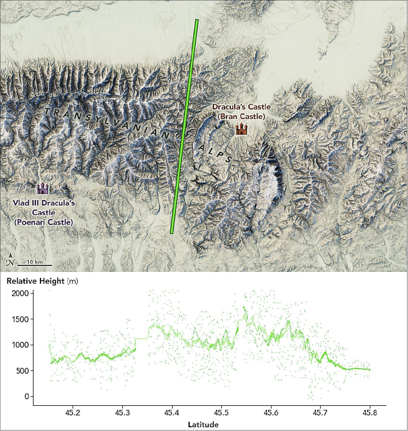
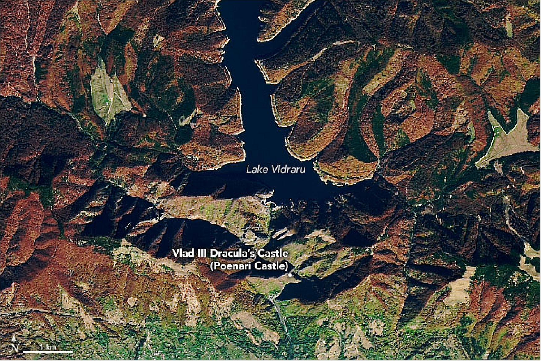
• October 18, 2019: Lake Mead, a reservoir along the Colorado River at the Arizona-Nevada border, can hold more water than any other reservoir in the United States. Full capacity, however, hasn’t been seen since 1983 due to drought and significant water usage. The decline is not constant: behind the Hoover Dam, water levels rise and fall with the seasons each year. 58)
- ATLAS measures elevation by sending pulses of light from the satellite to Earth’s surface. It then measures, to within a billionth of a second, how long it takes individual photons to return to the sensor. Each dot on the visualization above represents a photon detected by ATLAS. Most of the dots are clustered around the surface of the reservoir. Some penetrate the water—more in June, possibly due to smoother water that day. (Rough, wavy water scatters more photons, making it harder to penetrate the surface.)
- Notice that the lake’s surface elevation is quite a bit higher in spring (Figure 44). Most of the reservoir’s water comes from snowmelt from the Rocky Mountains, which in 2019 had an above average snow pack. Lake levels usually start to drop in late spring and early summer as water is drawn out for use by farms and cities in the American Southwest.
- The change matches well with ground-based measurements from the U.S. Bureau of Reclamation (USBR), which manages Lake Mead. Their data show that the lake’s water level dropped 5.53 feet (1.69 meters) between March and June. Still, June 2019 levels were the highest of any June since 2010.
- Despite the high snow pack and runoff in 2019, the USBR warned that the system of reservoirs in the Colorado River Basin is still strained and continues to be affected by a 20-year drought. The system’s reservoirs—of which Lake Mead and Lake Powell are the largest—are an important source of water for about 40 million people and 5.5 million acres (2,225,771 hectares) of farmland across the U.S. West and Mexico.
- ICESat-2 repeats its orbits every 91 days, making it useful for observing seasonal changes. The satellite was launched in September 2018, and as it accumulates more data over the years, annual patterns will begin to emerge. That’s particularly important for places that are more remote or not monitored from the ground.
- According to Lori Magruder, a research scientist at the University of Texas and the ICESat-2 science team lead: “Being able to quantify lake levels is huge in terms of tracking our planet’s water storage and monitoring how the change might fluctuate from year to year due to climate dynamics.”
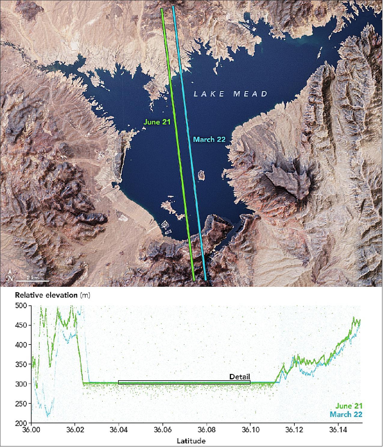
![Figure 44: Relative elevation of Lake mead in the period March 22 - June 21, 2019 [image credit: NASA Earth Observatory, image by Joshua Stevens, using ICESat-2 data courtesy of Kaitlin Harbeck (NASA/GSFC)]](https://www.eoportal.org/ftp/satellite-missions/i/ICESat2_290622/ICESat2_Auto26.jpeg)
• September 16, 2019: Photon Phriday is a weekly look at what ICESat-2 is measuring as it orbits the Earth. ICESat-2 Project Scientist Tom Neumann takes a look back at some recent passes in celebration of the first year on orbit for the mission. Follow @NASA_ICE for new Photon Phridays and results from NASA's ice-observing missions. 59)
• July 29, 2019: For nearly a year, the Advanced Topographic Laser Altimeter System (ATLAS) on NASA’s Ice, Cloud and land Elevation Satellite-2 (ICESat-2) has been measuring the height of Earth’s surfaces in remarkable detail—down to about 10 vertical centimeters. The elevation measurement above from Crater Lake in south-central Oregon was acquired by ATLAS on June 24, 2019, and shows what is possibly the instrument’s first overflight of a volcano. 60)
- The elevation data show the distinct topography of Mount Mazama and the crater lake that fills its caldera. For reference, the elevation track has been laid over a map of the lake and surrounding terrain. The map shows land cover, derived from a Landsat-based dataset, overlaid on a map of the topography as observed by NASA’s Shuttle Radar Topography Mission (SRTM).
- Moving from left to right (south to north), you can see the elevation increase gently and then more steeply up the flank of the volcano. The smaller-scale bumps are mostly tree tops. Where most satellite images offer a two-dimensional view of land cover, ICESat-2 provides a third dimension: tree height.
- The track next crosses Sun Notch—a classic u-shaped valley that was carved by glaciers during the formation of the mountain. Some valleys were filled with lava during periods of eruptions. Others, including Sun Notch, escaped that fate. Hikers today can walk through this valley to the Sun Notch overlook on the crater’s southern rim.
- The elevation then plummets hundreds of meters from the rim to the surface of Crater Lake. The 8- to 10-kilometer-wide caldera is the result of an enormous eruption and mountain collapse about 7,700 years ago. The lake that now fills the caldera is more than 580 meters (1,900 feet) deep, filling about half of the caldera’s depth. Crater Lake is the deepest lake in the United States, and the ninth deepest on Earth. The lake is too deep to see the bathymetry (ICESat-2 can measure bathymetry to a depth of 10 meters or more), but measurements of its surface elevation could be of interest to hydrologists.
- “This transect highlights how ICESat-2 elevation measurements provide interesting observations to a diverse number of scientists,” said Lori Magruder, a scientist at the University of Texas and the ICESat-2 science team lead. “Terrestrial ecologists would be interested in looking at the terrain around the lake as an indication of habitat quality. Others might investigate the vegetation to link the canopy heights to biomass estimates. Finally, the hydrologist would be interested in the lake level as an indicator of rainfall, groundwater flow, or evaporation.”
- Since ICESat-2 data were made available to the public in May 2019, scientists have started applying it to the mission objectives of measuring ice sheet elevation change, sea ice freeboard, and vegetation canopy height. Within the first six weeks of the the data release, more than 350 users made about 500,000 data downloads, and those data are already starting to show up in the scientific literature.
- “ICESat-2 is rapidly approaching one year on orbit, and the ATLAS instrument and spacecraft remain in nearly perfect working order,” said Tom Neumann, ICESat-2 project scientist at NASA’s Goddard Space Flight Center. “The initial data form ICESat-2 and its ATLAS laser instrument are exceeding scientists expectations.”
![Figure 46: Elevation data show the distinct topography of Mount Mazama and the crater lake that fills its caldera [image credit: NASA Earth Observatory image by Joshua Stevens, using ICESat-2 data courtesy of Kaitlin Harbeck (NASA Goddard Space Flight Center), Landsat data from the U.S. Geological Survey, and topographic data from the Shuttle Radar Topography Mission (SRTM). Story by Kathryn Hansen]](https://www.eoportal.org/ftp/satellite-missions/i/ICESat2_290622/ICESat2_Auto25.jpeg)
• July 29, 2019: Far more accurate than any previous map, this new representation of glacier flows in Antarctica opens the door to an improved understanding of the vast continent and the future pace of sea level rise. To create the new map, researchers at the University of California, Irvine, and NASA's Jet Propulsion Laboratory in Pasadena, California, combined input from six different satellite missions dating from 1994 to the present. 61)
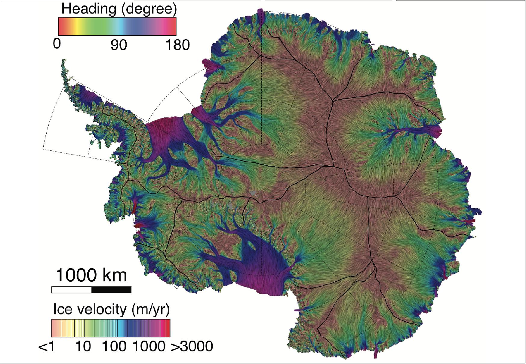
- All earlier maps of glacier flow speeds have estimated the speeds largely by tracking the movement of visible features like patches of dirt on the ice surface, but these new maps rely mainly on observations that use a technique called synthetic aperture radar interferometry, which is much more sensitive to the motion of the ice itself. By combining observations from multiple satellites passing over the continent in different directions, the researchers produced a map that is not only 10 times more accurate than any previous map but also shows speeds for far more of the slow-moving ice on the continental interior than ever before. 62)
- Constructed from a quarter century’s worth of satellite data, a new map of Antarctic ice velocity by glaciologists from UCI (University of California, Irvine) and NASA’s Jet Propulsion Laboratory is the most precise ever created. 63)
- “By utilizing the full potential of interferometric phase signals from satellite synthetic-aperture radars, we have achieved a quantum leap in the description of ice flow in Antarctica,” said lead author Jeremie Mouginot, UCI associate researcher in Earth system science. “This more detailed representation will help improve our understanding of ice behavior under climate stress over a larger part of the continent, farther south, and will enable improved projections of sea level rise through numerical models.”
- To chart the movement of ice sheets across the surface of the enormous land mass, the researchers combined input from six satellite missions: the Canadian Space Agency’s Radarsat-1 and Radarsat-2; the European Space Agency’s Earth remote sensing satellites 1 and 2 and Envisat ASAR; and the Japan Aerospace Exploration Agency’s ALOS PALSAR-1.
- While the data were spread across 25 years, the pace of signal gathering accelerated in the last decade as more resources were deployed in the Earth’s orbit. As ice sheet science coordinator in the World Meteorological Organization’s Polar Space Task Group, co-author Bernd Scheuchl, UCI associate project scientist in Earth system science, was responsible for acquiring the relevant data from the various international space agencies.
- Previous mapping efforts relied heavily on “feature” and “speckle tracking” methods, which detect the subtle motion of parcels of ice on the ground over time; this approach has been proven effective in estimating ice flow speed. To measure significantly slower ice sheet movement in the vast interior regions, the UCI team augmented these techniques with synthetic-aperture radar phase interferometry, which detects the subtle motion of natural reflectors of radar signals in snow/ice independent of the size of the parcel of ice illuminated by the radar.
- “The interferometric phase of SAR data measures the ice deformation signal with a precision of up to two orders of magnitude better than speckle tracking,” Mouginot said. “A drawback is that it requires a lot more data, namely multiple passes at different angles over the same point on the ground – a problem that was solved by a consortium of international space agencies pointing Earth-monitoring spacecrafts to this part of the world.”
- The team was able to compose a map that resolves ice movement to a level of 20 cm/year in speed and 5 degrees in annual flow direction for more than 70 percent of Antarctica. It’s the first time that high-precision mapping of the interior areas has been accomplished.
- “This product will help climate scientists achieve a number of goals, such as a better determination of the boundaries between glaciers and a thorough evaluation of regional atmospheric climate models over the entire continent,” said co-author Eric Rignot, chair and Donald Bren Professor of Earth System Science at UCI and a JPL senior research scientist.
- “It will also help in locating the most promising sites for ice core drilling to extract climate records and in examining the mass balance of Antarctica beyond its periphery.”
- He said he’s looking forward to the joint NASA and Indian Space Research Organization satellite, NISAR, launching in late 2021, which will be the first interferometric-mode SAR mission designed to look solely toward the South Pole. The spacecraft will provide a coast-to-coast view of Antarctica every 12 days.
- “We’ll be able to collect enough quality phase data over the Antarctic to generate updates to the map we just created in one or two months instead of one or two decades,” Rignot said. “With this level of precision in the interior regions, we’ll be able to reconstruct high-resolution spatial details in the bed topography beneath the ice through inversion techniques over far broader areas than in previous attempts – essential to improving ice sheet models and projections of sea level rise from Antarctica.”
- The new Antarctic ice velocity map and related datasets are available for download at the NASA Distributed Active Archive Center at the National Snow & Ice Data Center. This project was supported by NASA’s MEaSUREs program.
• May 28, 2019: More than a trillion new measurements of Earth’s height – blanketing everything from glaciers in Greenland, to mangrove forests in Florida, to sea ice surrounding Antarctica – are now available to the public. With millions more observations added each day, data from NASA’s Ice, Cloud and land Elevation Satellite-2 is providing a precise global portrait of elevation and will allow scientists to track even the slightest changes in the planet’s polar regions. 64)
- “The data from ICESat-2 are really blowing our minds, and I’m really excited to see what people with different perspectives will do with it,” said Lori Magruder, a senior research scientist at the University of Texas, Austin, and the ICESat-2 science team lead.
- The long-awaited ICESat-2 mission, launched in September 2018, continues the record of polar height data begun with the first ICESat satellite, which operated from 2003 to 2009. NASA’s airborne Operation IceBridge project bridged the data gap between the two satellites. The new satellite provides far more measurements than its predecessor. ICESat took approximately 2 billion measurements in its lifetime, a figure ICESat-2 surpassed within its first week.
- When ICESat orbited over a rift in Antarctica’s Filchner-Ronne Ice Shelf in October 2008, for example, it recorded a handful of data points indicating a crevasse in the ice. When ICESat-2 passed over 10 years later, it collected hundreds of measurements tracing the sheer walls and jagged floor of the growing rift.
- ICESat-2 is taking these measurements in a dense grid across the Arctic as well as Antarctica, recording each spot every season to track both seasonal and annual changes in ice.
- ICESat-2’s ability to measure heights beyond the poles is also impressing scientists – Magruder pointed to coastal areas, where in clear waters the satellite can detect the seafloor up to 30 m below the surface. Over forests, the satellite not only detects the top of the canopy, but the forest floor below – which will allow researchers to calculate the mass of vegetation in a given area.
- All this is being done with six laser beams from a satellite 500 km in space, noted Tom Neumann, ICESat-2 project scientist at NASA’s Goddard Space Flight Center in Greenbelt, Maryland.
- “Getting the exact latitude, longitude, and elevation of where a photon bounced off Earth is hard – lots of things have to happen and go really, really well,” he said. To make sure everything is working, the science team conducts a series of checks using data from airborne surveys, ground-based campaigns, even the satellite itself.
- That includes scientists travelling to Antarctica, where they drove modified snow-groomers along an arc of the 88-degree-south latitude line, taking highly accurate elevation measurements to compare with the data collected by ICESat-2 in space. Magruder compared measurements taken in White Sands, New Mexico, with what the satellite was tracking. In its most recent Antarctic and Arctic campaigns, NASA’s airborne Operation IceBridge flew specific routes designed to take measurements over the same ice, at close to or exactly the same time the satellite flew overhead.
- ICESat-2 is designed to precisely measure the height of ice and track how it changes over time. Earth’s melting glaciers cause sea levels to rise globally, and shrinking sea ice can change weather and climate patterns far from the planet’s poles.
- Small changes across vast areas like the Greenland ice sheet can have large consequences. ICESat-2 will be able to measure the shift in annual elevation across the ice sheet to within a fraction of an inch. To do this, the satellite uses a laser altimeter – an instrument that times how long it takes light to travel to Earth’s surface and back. With that time – along with the knowledge of where in space ICESat-2 is, and where on Earth the laser is pointing – computer programs create a height data point. The data is originally processed at NASA Goddard, then turned into advanced data products that researchers will be able to use to study elevations across the globe.
- ICESat-2 data products are now available for free from the National Snow and Ice Data Center at https://nsidc.org/data/icesat-2.
- For more information, visit www.nasa.gov/content/goddard/icesat-2 or https://icesat-2.gsfc.nasa.gov/. For more information on the data products, visit: https://earthdata.nasa.gov/icesat-2-data
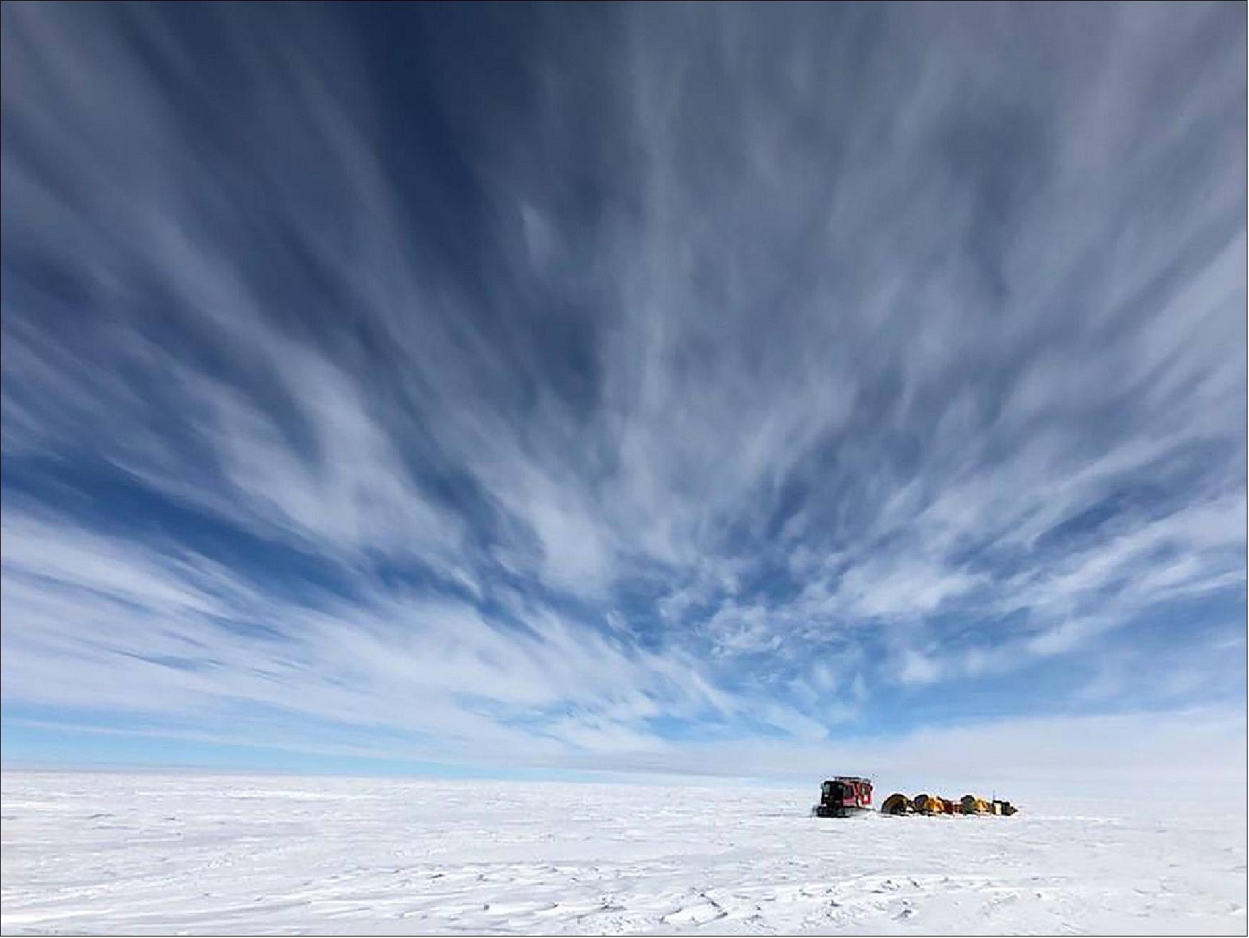
• January 29, 2019: NASA's ICESat-2 was launched in September 2018 and became the highest-resolution laser altimeter ever operated from space. The satellite is now measuring the height of Earth’s surfaces in remarkable detail. In this series, NASA Earth Observatory is sharing three early views that highlight the breadth of what ICESat-2 can “see”—from Antarctica’s icy terrain and sea ice to the forested landscape in Mexico. 65)
- The ICESat-2 satellite is already changing the way we look at Earth’s polar ice. But the satellite also collects detailed elevation measurements over tropical and temperate latitudes, providing a remarkable look at the heights of land and ocean features.
- ATLAS (Advanced Topographic Laser Altimeter System) measures elevation by sending pulses of light to Earth’s surface. It then measures, to within a billionth of a second, how long it takes individual photons to return to the sensor. Each dot on the visualization above represents a photon detected by ATLAS. Most of the dots in this “photon cloud” are clustered around a surface, whether that’s a tree top, the ground, or waves in the ocean.
- Along this orbital path from north to south (left to right of Figure 50) you first see a vegetated hillside sloping down toward the coastline. ICESat-2 can distinguish not only the tops of trees but also the inner canopies and the forest floor. Eventually, tree height data collected globally will improve estimates of how much carbon is stored in forests.
- As the path continues past the coastline, photons returned from the seafloor become visible. Bathymetry measurements like this are possible in clear coastal areas, sometimes as deep as 25 meters. According to Lori Magruder, a research scientist at the University of Texas and the ICESat-2 science team lead, the measurements could help with storm surge modeling. “Seeing such extensive bathymetry was a pleasant surprise,” she said. “We didn’t anticipate that.”
- Finally, as the path moves beyond Laguna del Mar Muerto and over the Pacific Ocean, the surface of the water is visibly rougher and the photons trace the height of individual waves. With this kind of information, scientists can start to look at things like the frequency of surface waves and their structure.
- “We were all taken aback seeing the amazing detail from ICESat-2,” Magruder said. “On every surface, there was some amazing feature that we weren’t used to getting from the first ICESat.”
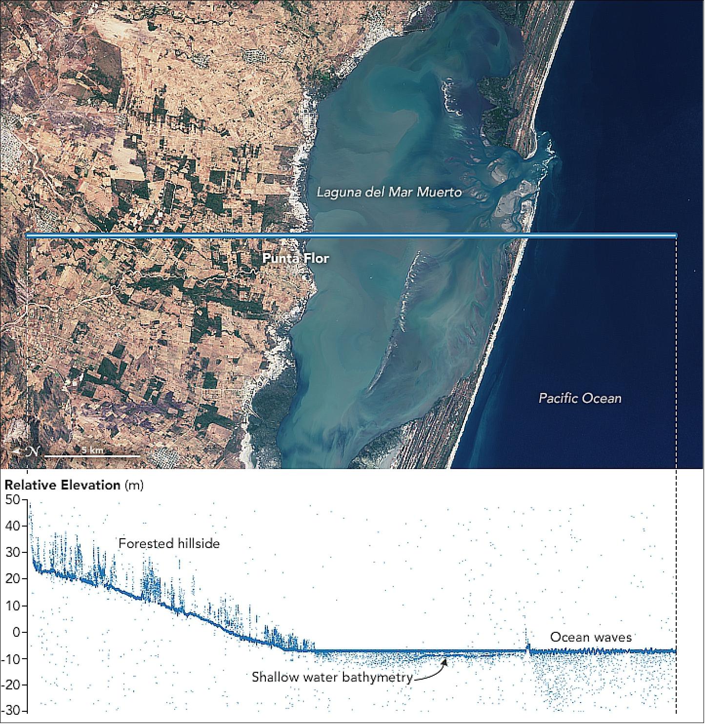
• December 12, 2018: NASA’s Ice, Cloud and land Elevation Satellite-2 (ICESat-2) was launched on 15 September 2018 and became the highest-resolution laser altimeter ever operated from space. The satellite is now measuring the height of Earth’s surfaces in remarkable detail. In this series, NASA Earth Observatory is sharing three early views that highlight the breadth of what ICESat-2 can “see.” 66)
- As scientists examined the first elevation data from the new ICESat-2 satellite, they saw vast, smooth stretches across Antarctica. Indeed, most of the continent’s snow- and ice-topped surface is flat. So too are the parts of an ice sheet that spread over the water, such as the Ross Ice Shelf. But there are some places where the terrain rises and falls steeply, such as the Transantarctic Mountains dividing East and West Antarctica.
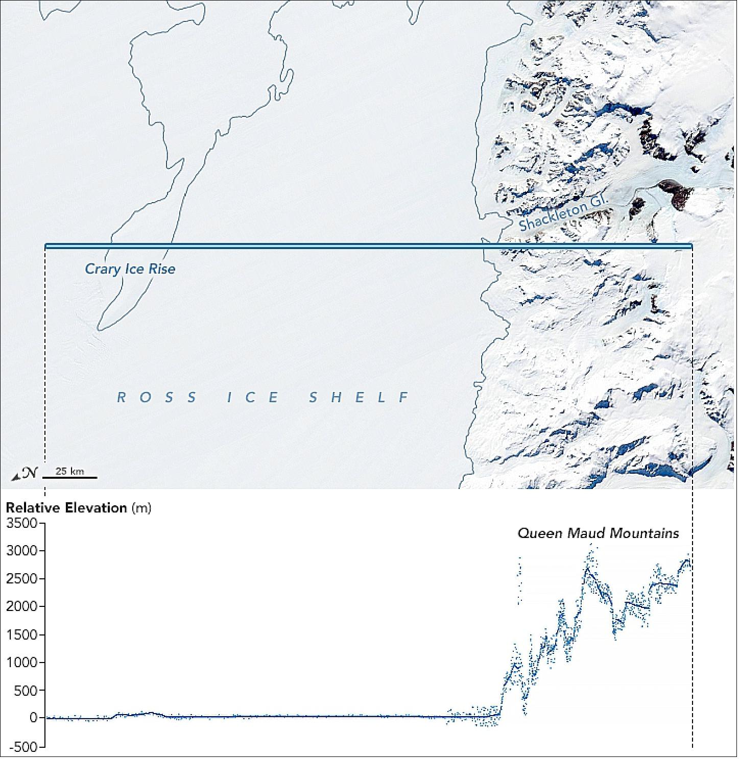
Legend to Figure 51: The rugged terrain of the Queen Maud Mountains—a subdivision of the Transantarctic Mountains—is visible in the elevation measurement, acquired on October 26, 2018, by ATLAS (Advanced Topographic Laser Altimeter System) on ICESat-2. For reference, the orbital path is laid over a natural-color image acquired on 23 November 2018, by the MODIS (Moderate Resolution Imaging Spectroradiometer) instrument on NASA’s Terra satellite.
- The ATLAS instrument measures elevation by sending pulses of light to Earth’s surface. It then measures, to within a billionth of a second, how long it takes individual photons to return to the satellite. Each dot on the visualization of Figure 51 represents a photon detected by ATLAS. Some of the dots in this “photon cloud” are photons from the Sun that reflected from the snow, but the densest areas form a line that indicate the height of a surface.
- “ICESat-2 can track the surface nicely over some difficult terrain. It can resolve small valleys in the mountains that are really hard to see in other altimetry data,” said Benjamin Smith, a glaciologist at the University of Washington. Some of these mountain slopes are very steep, with angles of more than 45 degrees. “Think about trying to stand up on something like that. It’s a pretty severe slope.”
- Not only is ICESat-2 showing more detail than previous space-based altimeters, it is also filling in existing gaps in coverage. Orbiting over more southern latitudes than ever before, the satellite can start to show changes closer to Antarctica’s center, where there are still large unknowns in how the ice is changing. Scientists think the changes are small, but the Antarctic Plateau is so vast that even very small changes to the height of the ice can lead to large changes in sea level.
- “Very soon we will have measurements that we can compare to older measurements from the first ICESat,” Smith said. ICESat flew from 2003 to 2010. “Then after a year we will have repeat measurements form ICESat-2 and can begin to watch ice sheets change in real time.”
• December 11, 2018: The first months of ICESat-2 data collected over Arctic and Antarctic sea ice reveal thin ice, thick ice, and features such as ice ridges. Areas of open water in the cracks between the ice floes, called leads, stand out in the data because of the difference in reflectivity between ice and water. By comparing the height of that water surface in the leads with the height of the ice, scientists are estimating ice freeboard and thickness. With the high precision of ICESat-2, plus the satellite’s six beams taking data simultaneously, researchers will have an unprecedented understanding of the thickness of sea ice, which will be used to help improve climate modeling and forecasts. 67)
- On thin ice: ”When sea ice first forms on polar oceans, before snow falls on it and wind smashes it into other floes, it is thin, flat and smooth. Which makes it a good place to test out how precise ICESat-2 data is, since long stretches should all be nearly the same height,” said Ron Kwok, a sea ice scientist at NASA’s Jet Propulsion Laboratory in Pasadena, California. So far? “The data’s spectacular,” Kwok said. “The fresh ice is totally flat to within a couple centimeters.”
- Plus, the ability to identify newly formed, thin ice will help researchers track the seasonal changes in remote polar regions, and understand the processes that drive those processes. The ice-thickness data will also help scientists improve computer models of how sea ice responds to Arctic warming, as well as forecasts of sea ice cover.
- “We’ll have much higher resolution of where it’s ice and where it’s water in the marginal ice zones, where the compact ice cover meets the ocean, during melt and freeze-up,” Kwok said. “That’s going to be new science to think about. “
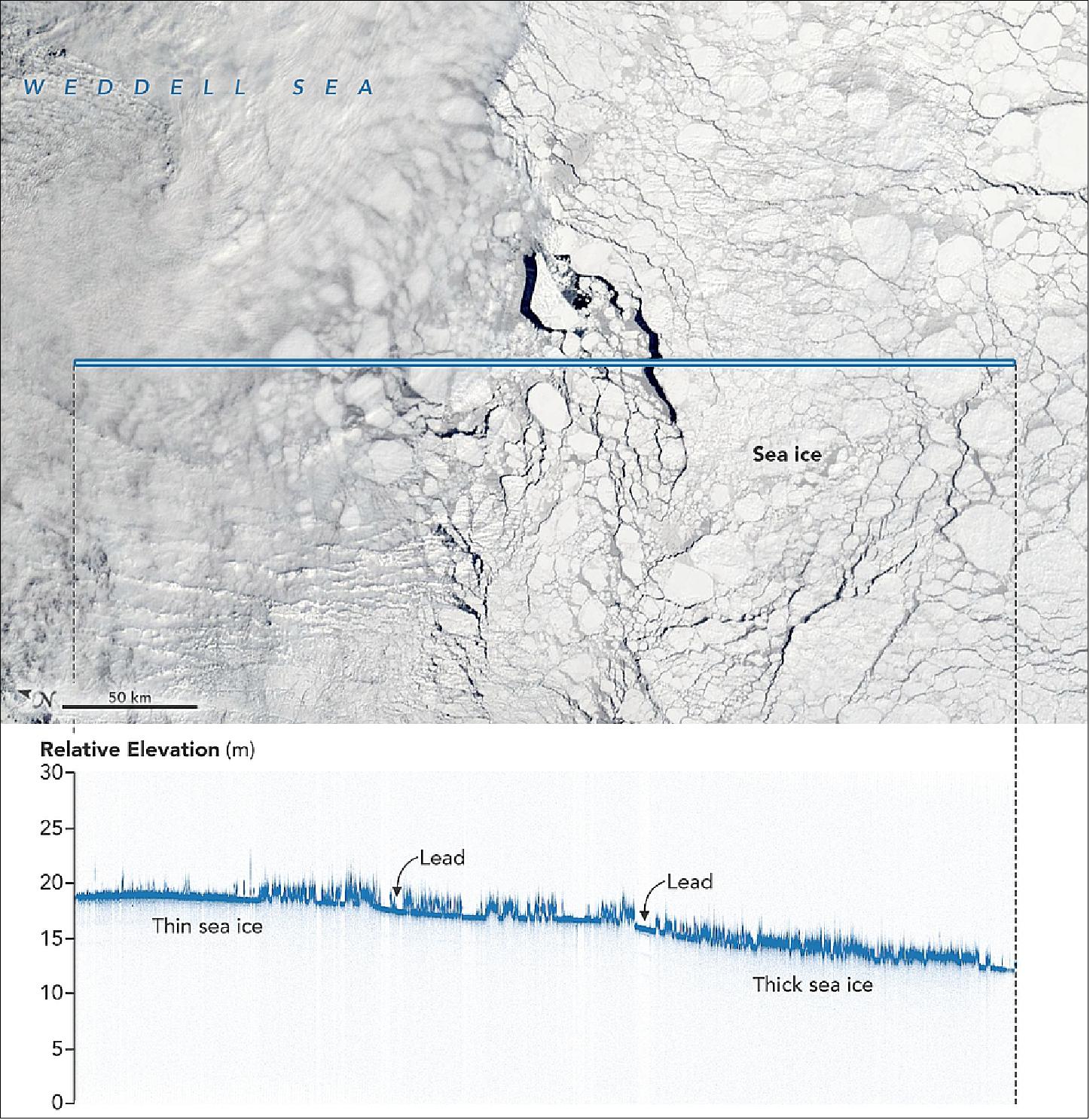
- Beyond ice: ICESat-2 is always on, taking measurements not only at the poles but also in the tropical and temperate latitudes, and what it can see has already surprised researchers.
- “We were all taken aback seeing the amazing detail from ICESat-2, thanks to its detection technology,” said Lori Magruder, a research scientist at the University of Texas and the ICESat-2 science team lead. “On every surface, there was some amazing feature that we weren’t used to seeing with the first ICESat.”
- For example, photons returning from over the ocean trace individual waves. In clear coastal areas, the bathymetry is visible, sometimes as deep as 25 meters, which could help with research including storm surge modeling, Magruder said.
- And as ICESat-2 orbits over forests, it can distinguish not only the tops of trees but also the inner canopies and the forest floor. While the team was unsure how clear the terrain would be under dense canopies like those found in tropical rainforests, the data turned out even better than expected. By measuring tree heights globally, the ICESat-2 mission will be able to improve estimates of how much carbon is stored in forests.
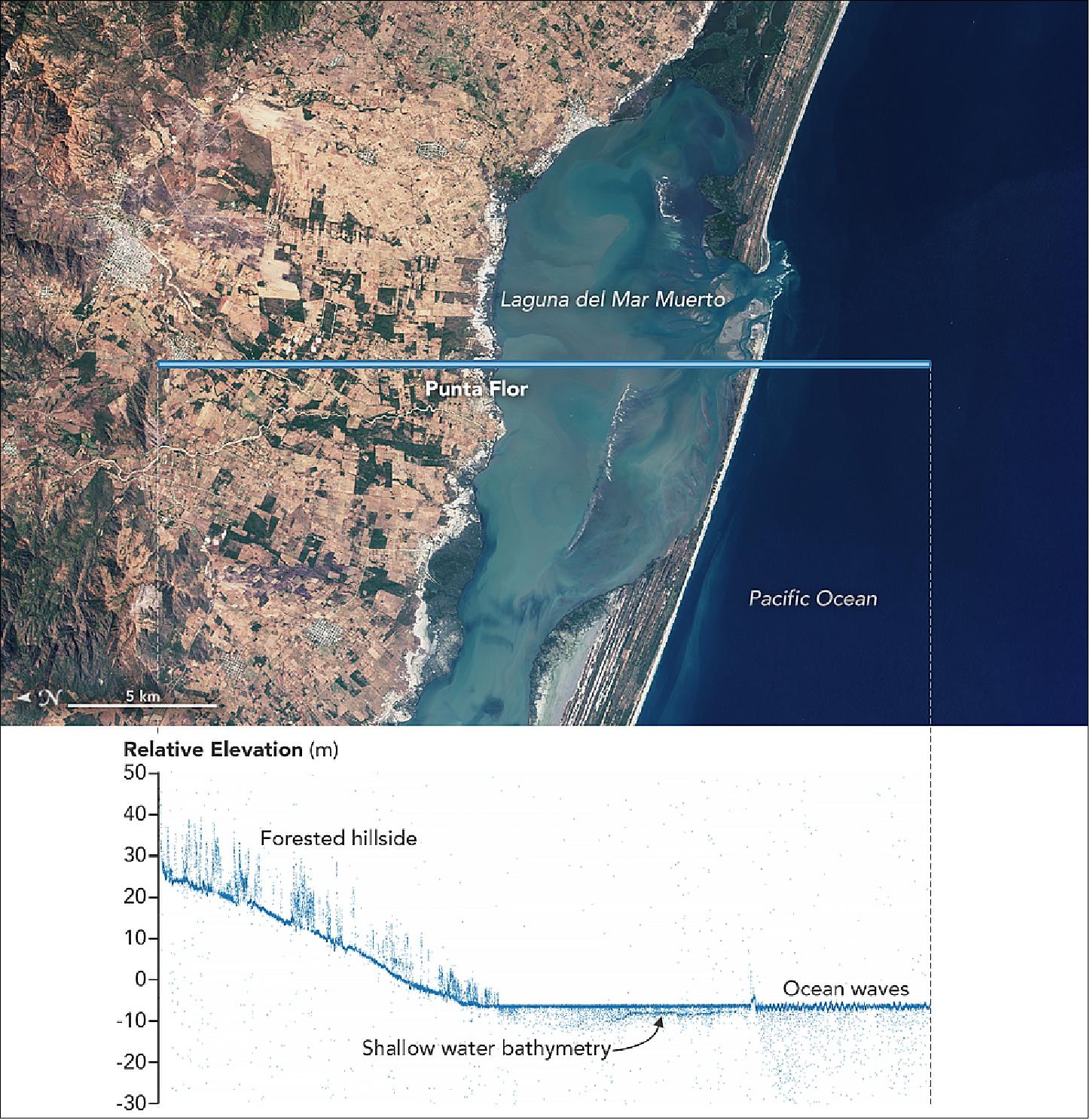
- Checking the numbers, bridging the gap: As the ICESat-2 science team was analyzing the first sets of data, colleagues with NASA’s Operation IceBridge were collecting data in aircraft over Antarctica – flying over the same paths that the satellite was orbiting.
- Over vast plains of rippling ice, craggy peaks poking through the ice sheet, and lines of crevasses marching down glaciers, the airborne campaign measured surface elevation with the Airborne Topographic Mapper’s laser altimeters, snow and ice thickness with radars, and sub-ice-shelf bathymetry with a gravimeter. For a decade, IceBridge has been surveying the region, but this fall they were also gathering data to help check the accuracy of ICESat-2.
- In three separate flights, IceBridge surveyed the flat plateau along the 88-degree-south latitude line where all ICESat-2 orbits converge. Other flights tracked across glaciers, ice streams and mountains along individual satellite paths – at times right as the satellite passed overhead. To measure sea ice, the IceBridge team flew briefly at 500 feet to measure wind speed, calculated how far the ice had moved since ICESat-2 measured it, and then adjusted the flight path to survey the same patch of ice.
- “Almost every flight has ICESat-2 tracks incorporated into it,” said Joseph MacGregor, IceBridge project scientist at NASA Goddard. “We fly over fast-changing outlet glaciers, the slower-changing interior, and uncommon surfaces that are interesting to ICESat-2. The primary goal for IceBridge is to bridge the gap between ICESat and ICESat-2, so it’s very rewarding to know that we’re completing that process.”
- The first ICESat satellite operated between 2003 and 2009, which is when IceBridge began its campaigns. ICESat-2 launched on 15 September from Vandenberg Air Force Base in California. Its laser instrument, called ATLAS (Advanced Topographic Laser Altimeter System), sends pulses of light to Earth. It then times, to within a billionth of a second, how long it takes individual photons to return to the satellite. ATLAS has fired its laser more than 50 billion times since first turning on Sept. 30, and all the metrics from the instrument show it is working as it should, Neumann said.
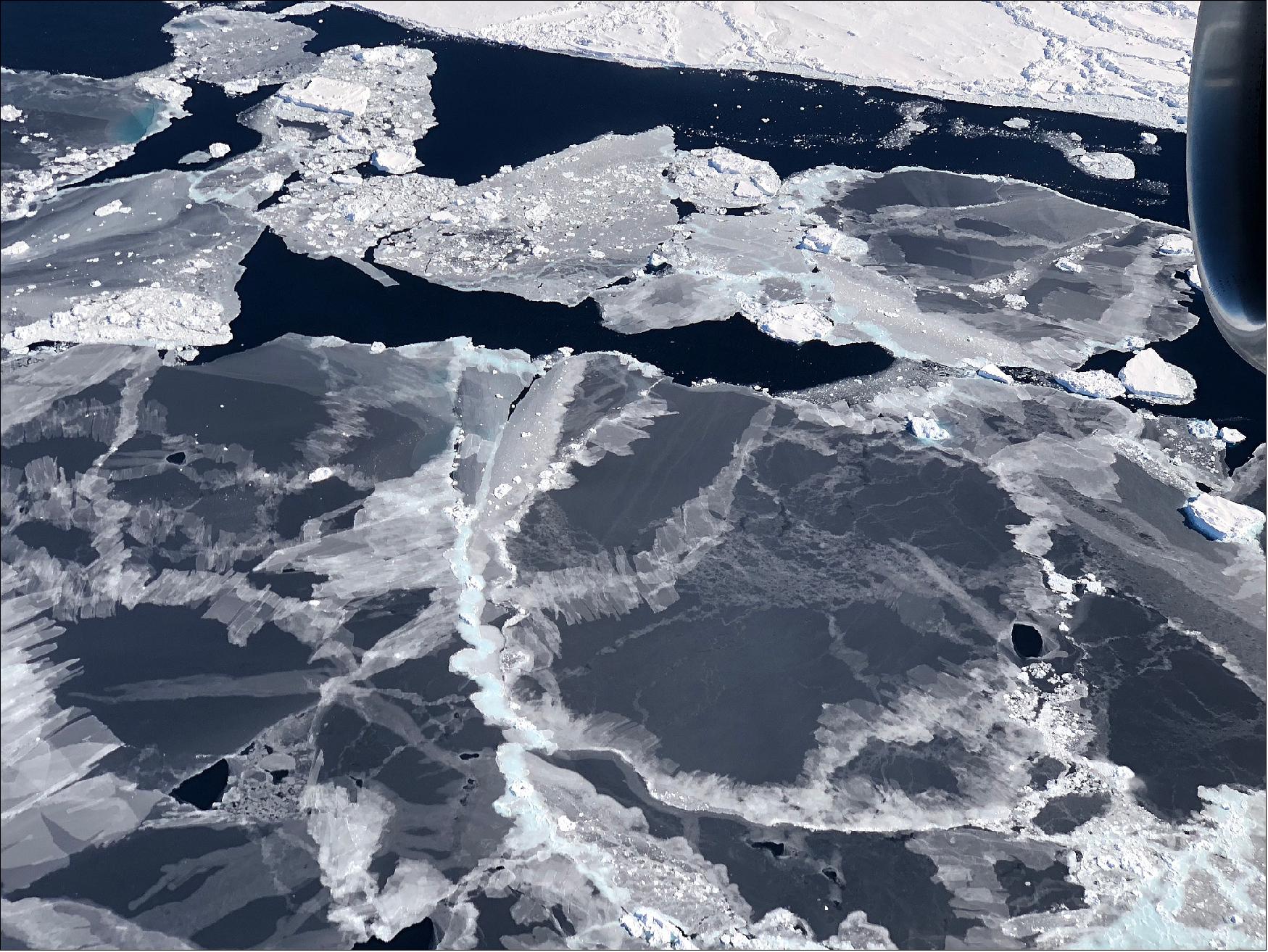
• October 3, 2018: The laser instrument that launched into orbit last month aboard NASA’s ICESat-2 (Ice, Cloud and land Elevation Satellite-2) fired for the first time on September 30. With each of its 10,000 pulses/s, the instrument is sending 300 trillion green photons of light to the ground and measuring the travel time of the few that return: the method behind ICESat-2’s mission to monitor Earth’s changing ice. By the morning of Oct. 3, the satellite returned its first height measurements across the Antarctic ice sheet. 68)
- “We were all waiting with bated breath for the lasers to turn on and to see those first photons return,” said Donya Douglas-Bradshaw, the project manager for ICESat-2’s sole instrument, called ATLAS (Advanced Topographic Laser Altimeter System). “Seeing everything work together in concert is incredibly exciting. There are a lot of moving parts and this is the demonstration that it’s all working together.”
- Once ICESat-2 was in space, the ATLAS team waited to turn on the lasers for about two weeks to allow any Earthly contaminants or gases to dissipate. “It’s very critical when you fire the lasers that you don’t have contaminants because you could damage the optics,” Douglas-Bradshaw said. “Fourteen days is well beyond the time needed for that, but we wanted to be safe.”
- During those two weeks, the ICESat-2 operations team turned on and tested the various systems and subsystems of the spacecraft and instrument, and fired thrusters to start placing the satellite in its final polar orbit, approximately 500 km above Earth.
- Before the laser was even turned on, however, the team eagerly awaited another milestone, Douglas-Bradshaw said. The door that protected the telescope and detector elements during launch had to be opened. The team had two chances to release one of two spring-loaded pins to open the door. This was successfully accomplished on 29 September.
- The following day, it was the laser’s turn. The engineering team had been working with the operations team that controls the instrument on orbit, so the commands were ready to go — first turning on the laser itself, waiting for it to warm up, and then issuing commands to put it in fire mode.
- The laser energy levels jumped up, and the device that starts ATLAS’s sophisticated stopwatch was active — two different, independent indicators that the laser was firing away. “We were all incredibly excited and happy, everyone was taking pictures of the screens showing data plots,” Douglas-Bradshaw said. “Someone noted: ‘Now we have a mission, now we have an instrument.’”
- Three days later, the ICESat-2 team had the first segment of height data, taken as the satellite flew over Antarctica.
- Computer programmers were up all night analyzing the latitude, longitude and elevation represented by each photon that returned to the ATLAS instrument — and by 6 a.m., Tom Neumann, ICESat-2 deputy project scientist, was texting screenshots of the height data to the rest of the team.
- “It was awesome,” Neumann said. “Having it in space, and not just simulating data on the ground, is amazing. This is real light that went from ATLAS to Earth and back again.”
- When scientists analyze the preliminary ICESat-2 data, they examine what is called a “photon cloud,” or a plot of each photon that ATLAS detects. Many of the points on a photon cloud are from background photons — natural sunlight reflected off Earth in the exact same wavelength as the laser photons. But with the help of computer programs that analyze the data, scientists can extract the signal from the noise and identify height of the ground below.
- The first photon cloud generated by ICESat-2 shows a stretch of elevation measurements from East Antarctica (Figure 55), passing close to the South Pole at a latitude of 88 degrees south, then continuing between Thwaites Glacier and Pine Island Glacier in West Antarctica.
- Next up for ICESat-2 is a suite of procedures to optimize the instrument, Neumann said, including tests to ensure the laser is pointing at the precisely correct angle and lasing at the precisely correct wavelength to allow as many photons as possible to hit the detector. “It will take a couple of additional weeks,” he said, “but about one month after launch we’ll hopefully start getting back some excellent science-quality data.”
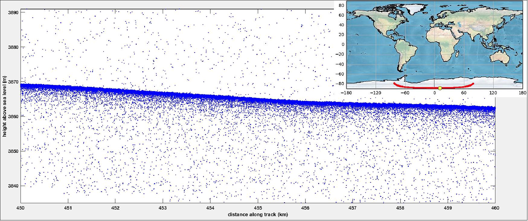
• September 15, 2018: Ground stations in Svalbard, Norway, acquired signals from the spacecraft about 75 minutes after launch. It’s performing as expected and orbiting the globe, from pole to pole (Ref. 27).
- “With this mission we continue humankind’s exploration of the remote polar regions of our planet and advance our understanding of how ongoing changes of Earth’s ice cover at the poles and elsewhere will affect lives around the world, now and in the future,” said Thomas Zurbuchen, associate administrator of NASA’s Science Mission Directorate.
ICESat-2 synergies with other atmospheric missions: 69)
ICESat-2 is expected to at least partially overlap with the operation of ADM/Aeolus and EarthCARE, during the 2018 to 2022 period. Overlap between ICESat-2 and CALIPSO and CATS is a bit more dubious: CALIPSO is already well beyond its projected mission lifetime and CATS (Cloud-Aerosol Transport System) on ISS has license to operate through February 2018, perhaps longer (it had a six-month requirement and three-year goal). There is, however, a possibility of a CATS “follow-on” mission (that would be known as CATS-I), which has been submitted in response to an Earth Venture Instrument-3 Announcement of Opportunity. Nevertheless, discussion on complimentary measurements during the meeting encompassed all instruments.
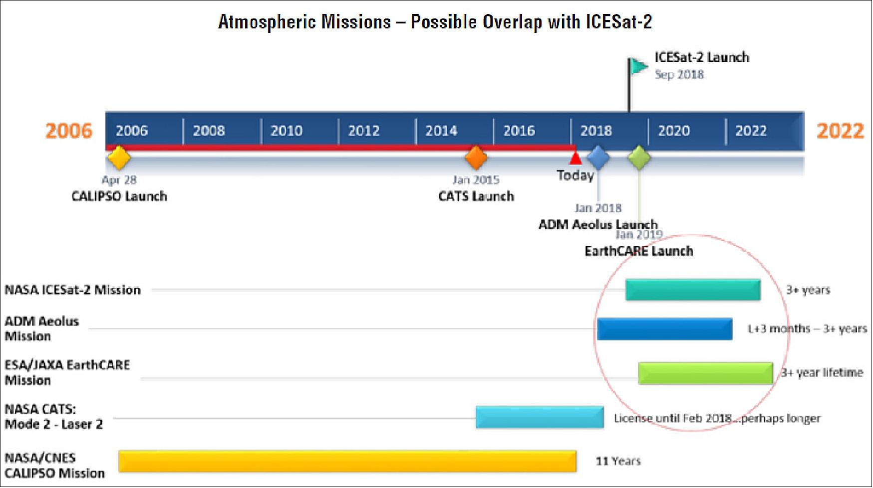
Sensor Complement
ATLAS (Advanced Topographic Laser Altimeter System)
ICESat-2 will use a new type of laser altimeter instrument, ATLAS, for measuring elevation, and will acquire far more data. To test the instrument concept, and develop accurate software to process the data, NASA has been flying an instrument called MABEL (Multiple Altimeter Beam Experimental Lidar) on high-altitude aircraft (ER-2) to simulate measurements that the ATLAS (Advanced Topographic Laser Altimeter System) — GLAS’s successor–will be making from space. 70) 71)
ATLAS instrument science measurement requirements (Ref. 75)
Land Ice: Ice‐sheet elevation changes to 0.4 cm/yr accuracy on an annual basis.
- Annual surface elevation change rates on outlet glaciers to better than 0.25 m/yr over areas 100 km2 for year‐to‐year averages.
- Surface elevation change rates to an accuracy of 0.4 m/yr along 1 km track segments for dynamic ice features that are intersected by the ICESat‐2 set of repeated ground‐tracks.
- Resolution of winter (accumulation) and summer (ablation) ice‐sheet elevation change to 10 cm at 25 km x 25 km spatial scales.
Sea Ice: Monthly surface elevation measurements with a track density of better than 30 km poleward of 70º, to enable the determination of sea ice freeboard when sea surface references are available, under clear sky conditions, to an uncertainty of 3 cm along 25 km segments, for the Arctic Ocean and Southern Oceans.
Vegetation: ICESat‐2 shall produce elevation measurements that enable determination of global vegetation height to 3‐m accuracy at 1 km spatial resolution in vegetated area with canopy closures less than or equal to 75% under clear sky conditions.
MABEL and ATLAS are photon-counting laser altimeters, meaning they measure distance by detecting just a few photons from each laser pulse and timing their round-trip travel from satellite to earth and back extremely accurately. While GLAS used millions of photons to make a single distance measurement, MABEL and ATLAS gather a data set of just a few dozen photons at most, and produce a cloud of points describing the snow or land or vegetation surface structure. Sophisticated software will determine the location of the surface track, the tops of the tree canopy, or the amount of dust or fog in the air.
The original design of the ATLAS instrument for ICESat-2 evolved as a modified version of the ICESat GLAS instrument concept. More specifically, for ICESat-2, the original ATLAS design was a single-beam altimetry system with the laser transmitter operating at a slightly higher repetition rate (50 Hz), lower energy per pulse (50 mJ) and similar 6-7 ns pulse width at the near-infrared (NIR) wavelength of 1064 nm when compared to GLAS. These changes would have provided higher derating on the lasers and potentially longer mission life.
In 2009, the ATLAS instrument on ICESat-2 underwent a complete redesign during the pre-Phase A activities to accommodate more science objectives and incorporate recommendations from the ICESat-2 science workshop (June 2007). For ice sheets, improved pointing will reduce the uncertainty in the ice sheet elevations introduced by the cross-track surface slope. In addition, for land topography and vegetation, improved pointing will provide observations along exact repeat ground tracks, and sampling along uniformly spaced ground tracks will provide well-sampled grids of topography and biomass. Based on this and other recommendations, a new instrument concept was proposed and accepted by the ICESat-2 program. 72) 73) 74) 75) 76) 77) 78)
The new baselined instrument is a high repetition rate (10 kHz), micropulse laser altimeter system. GSFC has begun an in-house program to investigate various potential laser technologies to meet the laser requirements for the ATLAS instrument.
A single laser transmitter having sufficient laser energy will be split into multiple beams using a DOE (Diffractive Optical Element) similar to the one used on LOLA. The current instrument architecture consists of a 9-beam system arranged in a 3 x 3 configuration.
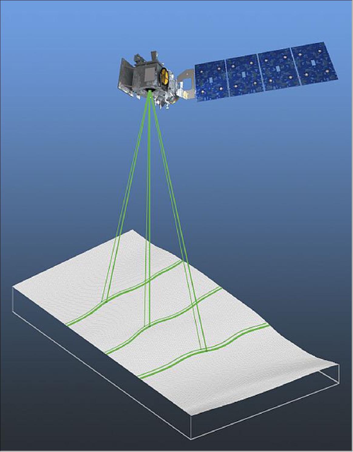
In contrast to the first ICESat mission, ICESat-2 will use micro-pulse multi-beam photon counting approach to provide:
- Dense cross-track sampling to resolve surface slopes on an orbit basis
- High repetition rate (10 kHz) generates dense along-track sampling (~70 cm)
- Different beam energies to provide necessary dynamic range (bright / dark surfaces)
The advantages are:
- Improved elevation estimates over high slope areas and very rough (e.g. crevassed) areas
- Improved lead detection for sea ice freeboard.
The ATLAS instrument is a multi-beam micropulse laser altimeter with the following features:
• Single laser beam split into 9 beams
• 10 m ground footprints
• 10 kHz repetition rate laser (~1 mJ)
• Multiple detector pixels per spot
• On-board boresight alignment system
• LRS (Laser Reference System) gives absolute laser pointing knowledge.
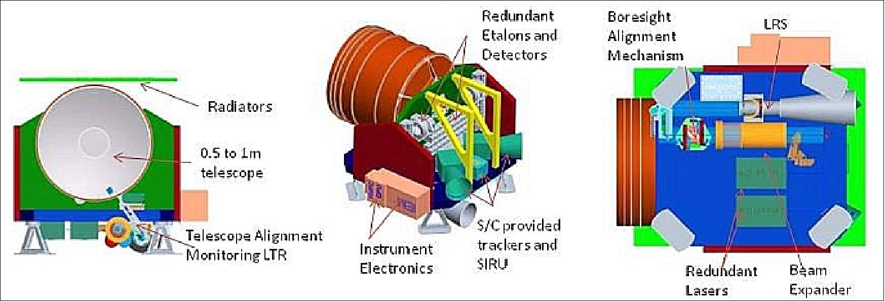
ATLAS will employ a micropulse laser transmitter frequency doubled to 532 nm (visible green) with a 1 ns FWHM pulse width and operating at a 10 kHz repetition rate (0.7 m along-profile footprint sampling). A narrow 20 µrad beam divergence from a 500 km orbit altitude will yield 10 m diameter footprints. To improve spatial sampling ATLAS will employ a DOE (Diffractive Optic Element) that will split the single transmit beam into 6 beams, creating a pattern consisting of 3 sets of 2 closely spaced (< 100 m) beams. The closely-spaced beam pairs will resolve local slope, enabling determination of real elevation change from a single repeat of a reference track (Ref. 4).
With ICESat-2 operating in a 91 day repeat orbit and ATLAS operating continuously, seasonal observations of inter-annual ice sheet elevation change will be possible. The beam pairs will be separated cross-track by 3 km, providing improved spatial coverage as compared to that of ICESat. Over land, rather than repeating reference tracks, spacecraft pointing will be used to systematically displace the profiles cross-track through time in order to build up dense global sampling of topography and vegetation over the course of the mission.
In the traditional analog Si:APD detection approach used by GLAS of ICESat-1, thousands of photons reflected from the Earth’s surface were acquired per laser fire (for clear atmospheric conditions) in order to obtain waveforms with sufficient SNR to achieve the 3 cm ranging precision. In the ATLAS micropulse approach the transmit pulse energy will be significantly lower such that only a few to ~10 photons will be detected per footprint per laser fire using a 0.8 m diameter telescope and photon-sensitive Photomultiplier Tube (PMT) detector arrays. Laser fire times and the arrival time of each photon, those reflected from the surface as well as from solar background noise, will be time tagged with 0.15 ns precision yielding < 20 cm single-photon range precision. Post-processing on the ground will yield “point clouds” of geolocated single photon surface returns. An advantage of this approach is that the combination of small, oversampled footprints, narrow pulse width and high-precision timing can yield elevation data of higher spatial and vertical resolution. In addition the geospatial information content of the point cloud is amenable to a greater diversity of analysis approaches than afforded by analog waveforms, opening up possibilities for new ways to characterize the vertical structure of the Earth’s surface (Ref. 4).
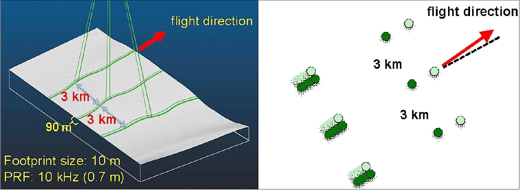
Legend to Figure 59: Single laser pulse, split into 6 beams. Redundant lasers, redundant detectors.
ATLAS carries two lasers on the optical bench – one primary and one backup. The laser light is at 532 nm, a bright green on the visible spectrum. It is fast-firing, sending 10,000 laser light pulses per second. 80)
The first step on the laser’s path to the ground is just a few inches past the laser, where a fold mirror directs the light 90º around a corner, where it hits the first key component, the PBC (Polarizing Beam Combiner). The PBC has two functions: The first is to make sure that the primary and backup lasers head down the same path. Although the two lasers won’t fire at the same time, the laser beams begin at different positions and need to end up at the same place. The second function is to use a periscope to pick off a fraction of the laser light and direct it to the LSA (Laser Sampling Assembly).
At the LSA, one of these fibers starts the ’stopwatch’ for that photon pulse. This timing component has to be incredibly precise to get the measurements that scientists need – when a photon returns, its travel time is recorded to the billionth of a second. The LSA also uses the small fraction of the laser to measure the laser’s wavelength, ensuring it remains precisely at 532.272 nm. This specific shade of bright green is what the filters on the receiving telescope let pass through to stop the stopwatch, once the laser pulse completes its journey. Any other wavelength gets filtered out as background noise. As the LSA starts the timer, the rest of the laser pulse continues to the BE (Beam Expander).
Shaping and steering the beam: The BE consists of two mirrors, facing each other but slightly angled so that the laser hits one, bounces across to the second one, and then continues on in the same direction. These mirrors are curved to make the laser beam more than four times wider once it bounces off them. Making the beam wider actually makes the photons diverge less as they travel to Earth, tightening the laser footprint on the ground and allowing for a more precise map of surface heights.
"The spot diameter on Earth’s surface would have been 66 m, now it’s 15 m," according to Ramos-Izquierdo. "By making the laser beam bigger in diameter before exiting the instrument, we actually decrease how much it spreads as it propagates downward through the atmosphere."
The wider laser beam now goes through the BSM (Beam Steering Mechanism), which directs the laser at the ground below, but also has fine control over where the laser is pointing. This mechanism is connected with components on the instrument's telescope receiver, which collects any photons that return. The goal is to automatically point the lasers at the exact spot on the ground, where the telescope is observing. If the telescope and laser are pointed at different spots, the BSM will make slight adjustments to correct the alignment. The BSM is key because as the satellite goes in and out of the sun, changes in temperature could slightly warp the optical bench.
Split in six: The last hurdle for the laser beam is the DOE (Diffractive Optic Element), on the far side of the beam steering mechanism. This optical component is etched with a microscopic pattern of crisscrossed lines, which splits the single laser beam into six. The beams are set at slightly different angles, so they will cover the ground in a specific formation of three pairs of beams.
Once through the Diffractive Optic Element, the photons – lined up perfectly in six beams – are off on their journey to Earth.
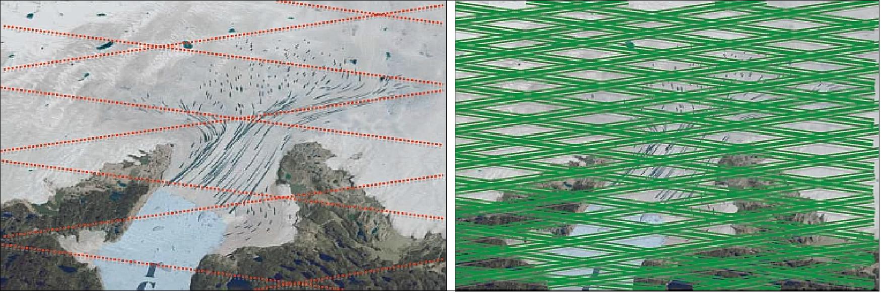
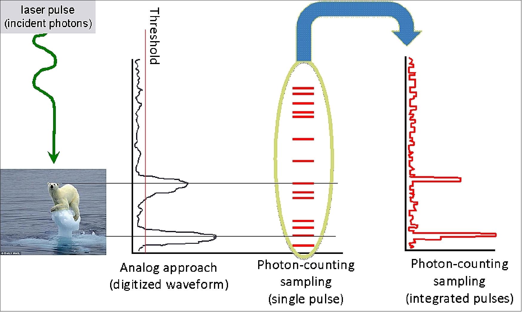
Legend to Figure 61: It is important to note that the integrated photon-counting sample (“histogram”) looks like the analog wave - but it is not - the information content is different, and the method of analyzing the data is different.
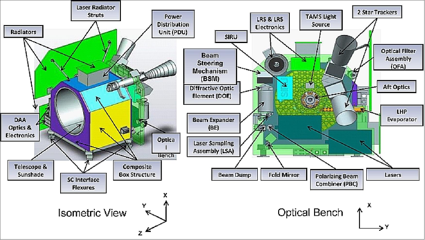
Pulse energy, pulse width | 2 mJ, < 1.5 ns |
PRF (Pulse Repetition Frequency) | 10 kHz (± 0.2 kHz) |
Center wavelength | 1020 - 1080 nm |
Wavelength stability/linewidth | < 60 pm |
PER (Polarization Extinction Ratio), polarization orientation | > 100:1, ± 1º |
Spatial mode | M2 < 1.6 |
Pointing stability (shot-to-shot), Pointing stability (long-term) | < 10% of divergence, < 20% of divergence |
Lifetime | > 5 years |
Operating temperature, operating survival temperature | ± 1ºC of design wavelength, 10 – 40ºC |
Non-operating survival temperature | 0 – 50ºC |
Design goals | |
Mass, volume, efficiency (wall plug) | < 10 kg, < 40 cm x 25 cm x 15 cm, > 15% |
Laser transmitter: The ATLAS laser represents a significant jump in space qualified laser technology (short pulse width, moderate average powers, frequency tunable and laser shot count). The ATLAS instrument is required to run continuously for 3 years on-orbit and the required laser shot count (~1 trillion) is ~3 orders of magnitude greater than in any previous NASA spaceflight mission. 81)
Fibertek Inc of Herndon, VA delivered three laser transmitters, including the one shown in Figure 63, that meet the demanding performance and reliability requirements for the ATLAS instrument, including two flight units and one spare. The lasers consists of two major sub-assemblies. The LOM (Laser Optical Module) is a sealed and pressurized module housing all of the optical components and laser diode modules. The LEM (Laser Electronics Module) is integrated to the LOM and is a vented module housing the laser power and command and control electronics.
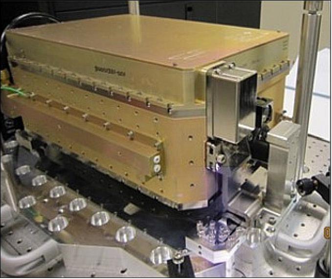
LOM (Laser Optical Module): A mature diode pumped solid Master Oscillator Power Amplifier (MOPA) architecture was selected in order to minimize schedule, cost and technical risks. End-pumped crystals gain heads are used in the oscillator and three subsequent amplifiers. The end-pumped gain heads are designed with methodology similar to mature geometries used broadly in commercial laser systems.
The master oscillator generates 200 µJ infrared pulses with <1.5 ns full width half max pulse widths with narrow (< 5 pm) linewidth tunable over a >50 pm wavelength range. The oscillator’s output is amplified via three stages to more than 1.8 mJ at 10 kHz pulse repetition frequency while preserving the near diffraction-limited beam quality (M2 < 1.4) and short pulse widths of the oscillator output. The 1064 nm amplifier output is frequency doubled to 532 nm via a critically phased matched lithium triborate (LBO) crystal.
The ATLAS lasers generate 532 nm output pulses with user-selectable energies from 250 µJ to 1.2 mJ with near-diffraction limited beam quality and < 1.5 ns pulse widths. Additional system design details have been previously published.
The ATLAS lasers systems successfully completed a protoflight qualification program including electromagnetic interference testing, vibration testing and thermal vacuum testing, specific testing details are published . In addition, three early system prototypes completed >25,000 hour life tests demonstrating the laser design was capable of meeting the mission operational run time requirement. A summary of the key laser requirements and achieved performance is listed in Table 3.
Parameter | Requirement | Flight Lasers |
Energy (µJ) | 250-900 | 250-1,370 |
Pulse rate (kHz) | 10 | 10 |
Divergence (µrad) | <130 | 91 |
Wavelength (nm) | 532.272 | 532.272 |
Linewidth (pm) | <30 | <5 |
Efficiency | >5% | 8.2% |
Operational run-time | 3.5 years (>1 trillion shots) | Prototype systems (>1 trillion shots) |
LEM (Laser Electronics Module): The electronic design was started early in the program mitigating design surprises and long lead Electrical, Electronic and Electromechanical (EEE) part procurement schedules. The integrated ATLAS electronics included the following major electronic boards.
Laser Control Board: Provides high speed communications with the payload, to monitor numerous laser health and diagnostic sensors (14 temperature sensors, four internal energy monitors, two pressure sensors, other housekeeping telemetry) while providing the critical timing parameters needed for a laser capable of 12 user selectable energy modes.
Diode Power Module: A custom high efficiency (>87%) DC-DC converter purpose built to provide power conditioning to four custom pulsed diode drivers.
Pulsed Diode Driver: Four pulsed diode drivers generating the programmable current waveforms with a peak current of 4 A, ~28 VDC at 10 kHz with µs class rise and fall times, and 85% efficiency.
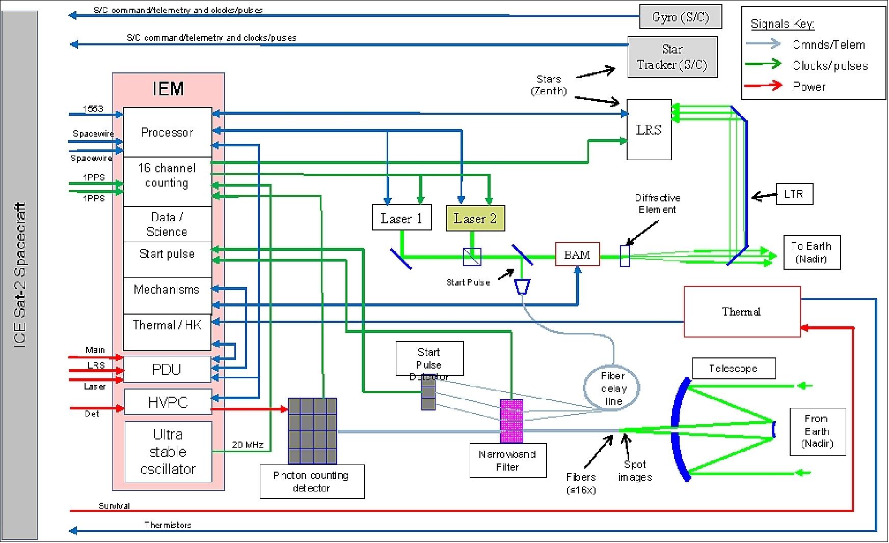
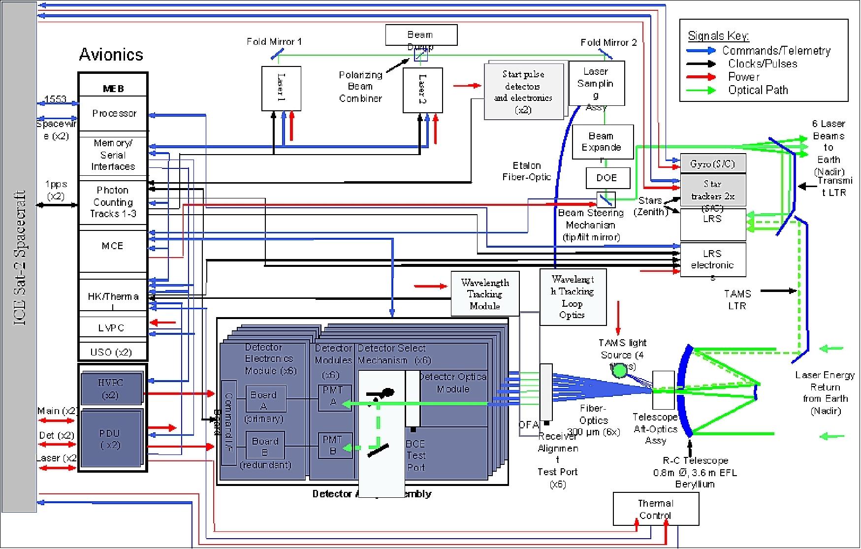
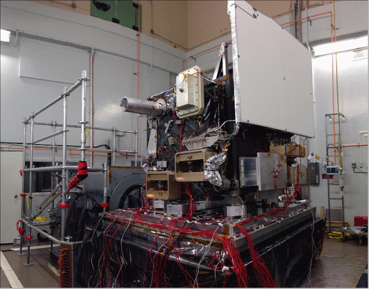
The ATLAS instrument has a mass of 298 kg and a power consumption of 300 W.
Ground Segment
Just as with the original ICESat data, ICESat-2 measurements are expected to provide added value to science and applications beyond their primary purpose. NASA’s Applied Sciences Program actively seeks to connect NASA’s Earth-observing satellite data to societal applications and encourages each mission to come up with a plan to connect its science to user needs. To that end, the ICESat-2 mission established an ICESat-2 Applications Team to organize and develop a mission applications program that will help establish these vital links between ICESat-2 science and society.
With guidance from the Applications Team, ICESat-2 has developed and implemented a diverse range of mission-specific prelaunch applications activities and strategies for engaging end users. These activities are modeled after the highly successful application strategies implemented for NASA’s SMAP (Soil Moisture Active/Passive) mission and are intended to provide a fundamental understanding of how ICESat-2’s data products can be best integrated into operational procedures to improve decision-making efforts across multiple disciplines. 82)
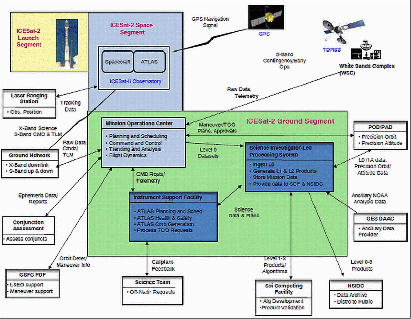
Product No | Product Name | Short Description | Latency |
ATL00 | Telemetry Data | Raw ATLAS telemetry in packet format. | Downlinked 8 times/day |
ATL01 | Reformatted Telemetry | Parsed, partially reformatted into HDF5, and generated daily. Segmented into several-minute granules. | 2 days |
ATL02 | Science Unit Converted Telemetry | Photon time-of-flight, corrected for instrument effects. Includes all photons, pointing data, spacecraft position, housekeeping data, engineering data, and raw atmospheric profiles. Segmented into several-minute granules. | 2 days |
ATL03 | Global Geolocated Photon Data | Precise latitude, longitude, and elevation for every received photon, arranged by beam in the along-track direction. Photons classified by signal vs. background, as well as by surface type (i.e., land ice, sea ice, land, ocean), including all geophysical corrections (e.g., Earth tides, atmospheric delay). Segmented into several-minute granules. | 21 days |
ATL04 | Calibrated Backscatter Profiles | Along-track atmospheric backscatter data —25 times per second. Includes calibration coefficients for polar regions. Segmented into several-minute granules. | 21 days |
ATL06 | Land Ice Height | Surface height for each beam with along- and across-track slopes calculated for each beam pair. Posted at 40 m along-track; segmented into several-minute granules. | 45 days |
ATL07 | Arctic/Antarctic Sea Ice Elevation | Height of sea ice and open water leads at varying length scale based on returned photon rate for each beam—pre-sented along-track. | 45 days |
ATL08 | Land Water Vegetation Elevation | Height of ground—including canopy surface—posted at fixed-length scale, for each beam presented along-track. Where data permit, include canopy height, canopy cover percentage, surface slope and roughness, and apparent reflectance. | 45 days |
ATL09 | ATLAS Atmosphere Cloud Layer Characteristics | Along-track cloud and other significant atmosphere layer heights, blowing snow, integrated backscatter, and opti-cal depth. | 45 days |
ATL10 | Arctic/Antarctic Sea Ice Freeboard | Estimate of sea ice freeboard over specific spatial scales using all available sea surface height measurements. Contains statistics of sea surface and sea ice heights. | 45 days |
ATL11 | Antarctica/Greenland Ice Sheet H(t) Series | Time series of height at points on the ice sheet—calculated based on repeat tracks and/or crossovers. | 45 days from receipt of last data in product |
ATL12 | Ocean Elevation | Surface height at specific length scale. Where data permit, include estimates of height distribution, roughness, surface slope, and apparent reflectance. | 45 days from receipt of last data in product |
ATL13 | Inland Water Elevation | Along-track inland water elevation based on specific inland water mask. Where data permit, include roughness, slope, and aspect. | 45 days from receipt of last data in product |
ATL14 | Antarctica/Greenland Ice Sheet H(t) Gridded | Height maps of each ice sheet for each year, based on all available elevation data. | 45 days from receipt of last data in product |
ATL15 | Antarctica/Greenland Ice Sheet dh/dt Gridded | Height change maps for each ice sheet, for each mission year, and for the whole mission. | 45 days from receipt of last data in product |
ALT16 | ATLAS Atmosphere Weekly | Polar cloud fraction, blowing snow frequency, and ground detection frequency. | 45 days from receipt of last data in product |
ATL17 | ATLAS Atmosphere Monthly | Polar cloud fraction, blowing snow frequency, and ground detection frequency. | 45 days from receipt of last data in product |
ATL18 | Land/Canopy Gridded | Gridded ground surface height, canopy height, and canopy cover estimates. | 45 days from receipt of last data in product |
ATL19 | Mean Sea Surface (MSS) | Gridded ocean height product. | 45 days from receipt of last data in product |
ATL20 | Arctic/Antarctic Gridded Sea Ice Freeboard | Gridded sea ice freeboard. | 45 days from receipt of last data in product |
ATL21 | Arctic/Antarctic Gridded Sea Surface Height within Sea Ice | Gridded monthly sea surface height inside the sea ice cover. | 45 days from receipt of last data in product |
ICESat-2 Preparatory Campaigns
NASA Operation IceBridge Campaign in Antarctica 2018
• October 23, 2018: Operation IceBridge, NASA’s longest-running aerial survey of polar ice, flew over the northern Antarctic Peninsula on Oct. 16, 2018. During the survey, designed to assess changes in the ice height of several glaciers draining into the Larsen A, B and C embayments, IceBridge senior support scientist Jeremy Harbeck spotted a very sharp-angled, tabular iceberg floating among sea ice just off of the Larsen C ice shelf. A photo of the iceberg (seen at right) was widely shared after it was posted on social media. 83)
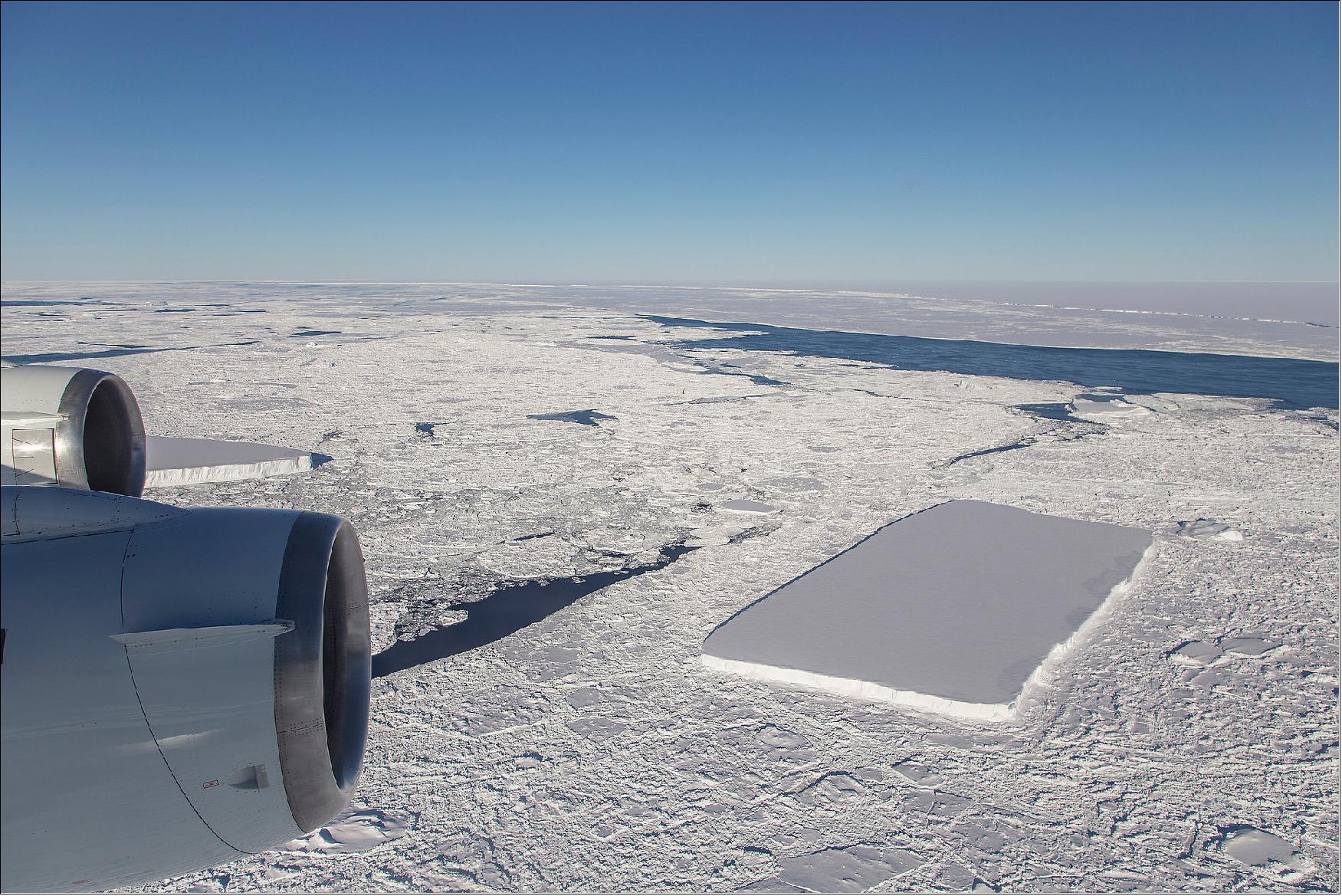
“I thought it was pretty interesting; I often see icebergs with relatively straight edges, but I've not really seen one before with two corners at such right angles like this one had,” Harbeck said. The rectangular iceberg appeared to be freshly calved from Larsen C, which in July 2017 released the massive A68 iceberg, a chunk of ice about the size of the state of Delaware.
• October 12, 2018: NASA’s decade-long airborne survey of polar ice, Operation IceBridge, is once again probing Antarctica. But this year is different: it is the first time that the IceBridge team and instruments survey the frozen continent while NASA’s newest satellite mission, the Ice, Cloud and land Elevation Satellite-2 (ICESat-2), studies it from space. 84)
After successfully flying over the Bailey Ice Stream and Slessor Glacier in East Antarctica on 10 October, IceBridge will spend the next five weeks measuring changes in Antarctic sea and land ice while precisely flying under orbits of ICESat-2 to compare measurements.
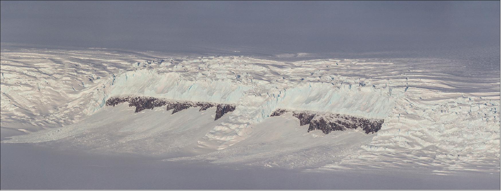
IceBridge began flying in 2009 to maintain continuity of laser-altimetry measurements between NASA’s ICESat missions. The original ICESat mission ended in 2009, and its successor, ICESat-2, was launched on 15 September 2018. Since then, ICESat-2 has successfully collected its first height measurements across the Antarctic Ice Sheet on 3 October.
“After a decade of flying both poles every year, we’re finally bridging the two ICESat satellite missions,” said Joe MacGregor, IceBridge’s project scientist and a glaciologist at NASA’s Goddard Space Flight Center in Greenbelt, Maryland. “It’s hugely satisfying to be part of building this key observational record of change in the polar regions.”
“This campaign is our second-to-last Antarctic campaign and it is arguably the most scientifically diverse that IceBridge has ever done,” MacGregor said. “We’re going to be revisiting classic IceBridge targets: flights along glacier flowlines that have been surveyed since 2002, long-term sea ice flights, and new targets across West Antarctica. More than two dozen of these mission designs are relevant to both IceBridge and ICESat-2.”
IceBridge and ICESat-2 both use laser altimeters that fire pulses of light toward the ground and measure how long it takes for that light to bounce off the ice and return to the instruments’ sensors. Scientists can then calculate the distance between the aircraft or the satellite and the ice surface, which gives them the ice height.
When IceBridge flies along a track over Antarctica that ICESat-2 has either just or is about to pass over as it orbits in space, pilots will align the plane so that the swath fired by IceBridge’s laser altimeter encompasses the tracks of two of ICESat-2’s six laser beams. Researchers will then look for overlap between the IceBridge and ICESat-2 returns and compare their measurements of ice height.
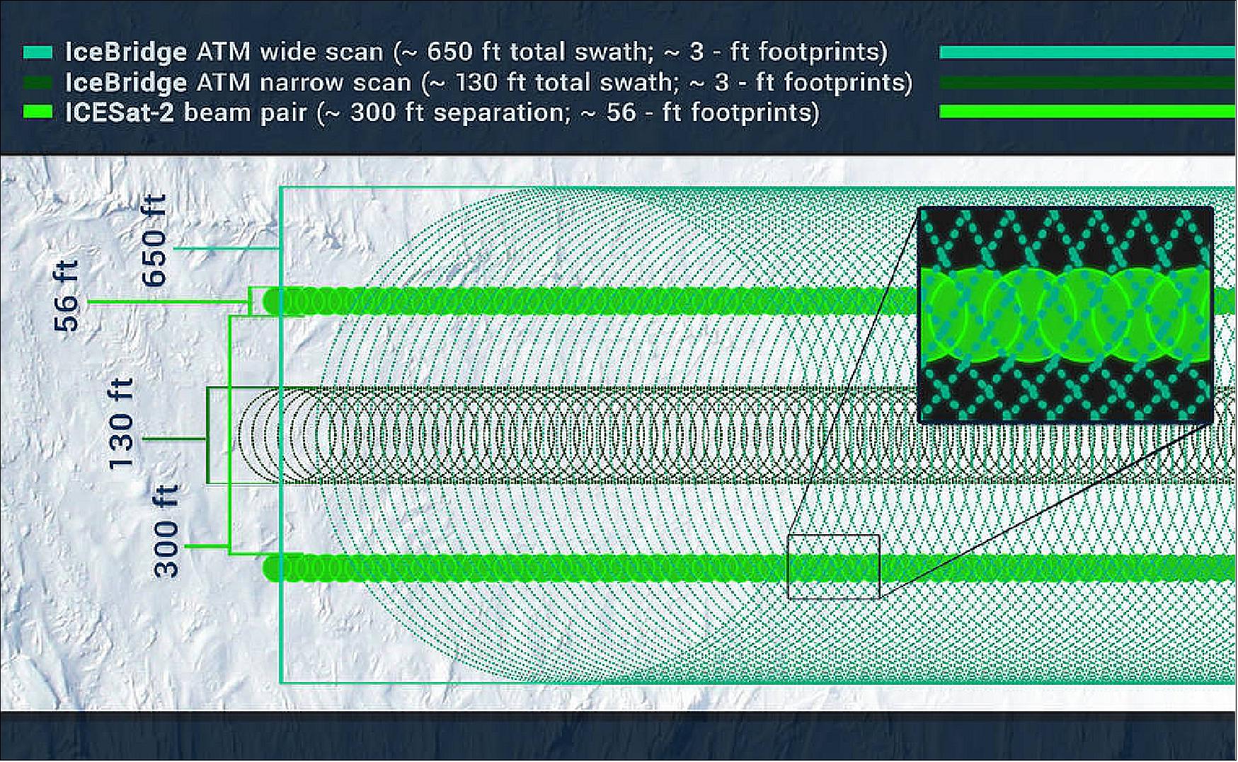
During this year’s Antarctic campaign, the IceBridge team will fly under some of ICESat-2’s orbits over sea and land ice. The underflights over sea ice to collect measurements of freeboard — the total height of the snow cover and sea ice that floats above the ocean — are particularly tricky. The ice that floats over the Southern Ocean is in constant motion, so in order to survey the same patches of sea ice that ICESat-2 will have flown over a few hours earlier or later that day, the IceBridge scientists will first have to figure out where that sea ice has drifted.
“We’re going to be chasing sea ice,” said Linette Boisvert, IceBridge’s deputy project scientist and a sea ice researcher at Goddard. “To do so, we will take the plane down to a lower altitude and remain there for a few seconds to measure wind speed and direction. We’ll plug these data into a code that accounts for drift and other forces, calculating where the sea ice that ICESat-2 flew over is currently located. Then, we’ll adjust our route to fly over it. On the way back to base, we’ll drop lower again to measure wind speed, readjust our trajectory and chase sea ice again.”
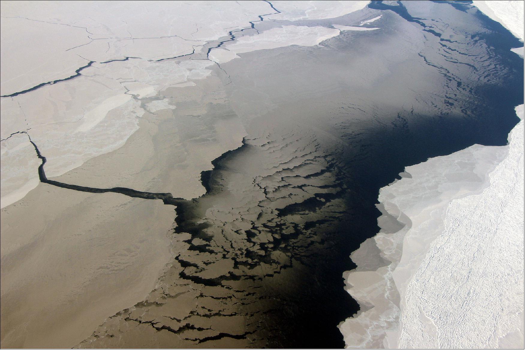
Another modification to meet ICESat-2’s needs will be performing a sea ice survey at twilight. Normally, IceBridge only conducts its flights in broad daylight, but, since ICESat-2 will be taking measurements around the clock, the scientists want to check whether laser data are more accurate at low light, when there is less interference on the laser instrument’s sensors from the Sun.
While flying over Antarctica, IceBridge will also collaborate with satellite missions and international research groups as weather and time allow. During the sea ice surveys, the IceBridge plane may also fly under the tracks of ESA’s (European Space Agency) CryoSat-2 and the European Union’s Sentinel-3 satellites. During a survey flight over Thwaites Glacier, one of the fastest-changing glaciers in West Antarctica, IceBridge may collect seafloor measurements to support the International Thwaites Glacier Collaboration, a joint campaign between the United States and the United Kingdom.
This year, IceBridge flights to Antarctica will begin first from Punta Arenas, in southern Chile, and later from Ushuaia, in southern Argentina. The surveys will be conducted from NASA’s DC-8 airborne science laboratory. The plane, managed by NASA’s Armstrong Flight Research Center in Palmdale, California, carries IceBridge’s full instrument suite.
IceBridge’s main instrument is a dual-color laser altimeter from NASA's Wallops Flight Facility in Virginia that measures surface elevation by transmitting both infrared and green laser pulses. The airborne mission also uses two types of radar systems from the Center for Remote Sensing of Ice Sheets at the University of Kansas to study ice layers and Antarctica’s bedrock. Wallops also contributes a high-resolution camera to collect color images of the ice surface and infrared cameras to read surface temperatures of sea and land ice. Goddard provides a hyperspectral imager to the mission that takes measurements over hundreds of wavelengths and Columbia University in New York manages a gravimeter to map the seafloor underneath the ice shelves.
MABEL (Multiple Altimeter Beam Experimental Lidar)
MABEL is a high-altitude airborne laser altimeter designed as a simulator for ICESat-2. The MABEL design uses multiple beams at fixed angles and allows for local slope determination. The MABEL instrument was developed to: 85) 86)
1) enable the development of ICESat-2 geophysical algorithms prior to launch
2) provide detailed error analysis of the ATLAS measurement strategy
3) provide ATLAS model validation.
MABEL is a photon-counting multibeam lidar sampling at both 532 nm and 1064 nm wavelengths using short (~1.5 ns) laser pulses. MABEL beams are arranged in a linear array, perpendicular to the direction of flight. The system allows for beam-geometry changes between flights with a maximum view angle of ±1 km from a 20 km nominal altitude achieved during the 2010–2012 deployments using a NASA ER-2 aircraft (Figure 73).
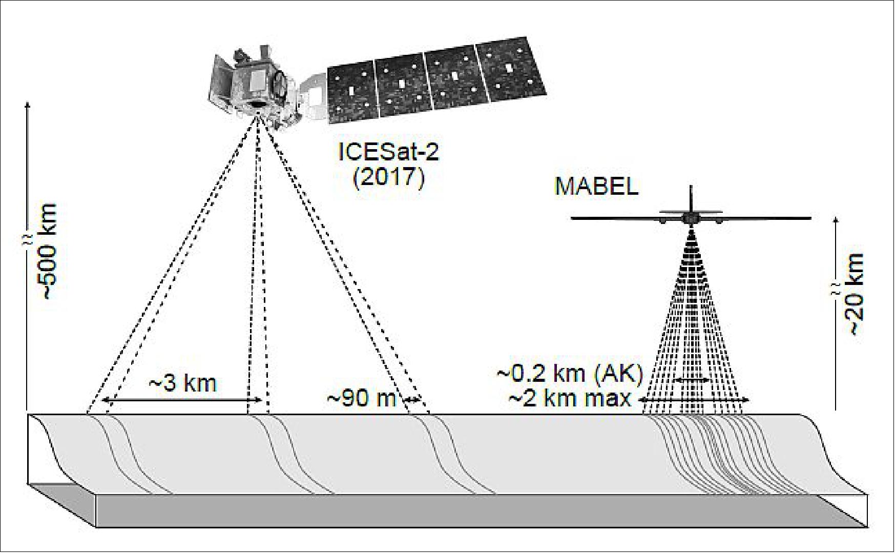
The repetition rate of MABEL is variable (between 5 and 25 kHz); most flights during the 2010–2012 deployments used 5 kHz. At this nominal altitude, repetition rate, and an aircraft speed of ~200 m/s, MABEL samples a ~2 m footprint every ~4 cm along track. During these initial MABEL deployments, beam geometry (specifically the spacing between the individual beams) was configured to mimic ICESat-2.
Following engineering test flights in December 2010 and March 2011, MABEL was deployed to Greenland in April 2012 to collect data over polar targets (Figure 74).
Operation IceBridge is a NASA airborne campaign intended to bridge the data gap between ICESat and ICESat-2. Operation IceBridge hosts a suite of instruments, including the ATM (Airborne Topographic Mapper). ATM is a lidar that conically scans at a rate of 20 Hz, with an off-nadir scanning angle of ~15º. Like GLAS, ATM digitizes returned energy as a waveform with derived surface elevations based on 532 nm wavelength pulses and a 5 kHz PRF (Pulse Repetition Frequency). The ATM flights were conducted using the NASA P-3B at an aircraft speed of ~100 m/s, with a nominal elevation of 500 m above ground level. At this air speed, elevation, and repetition frequency, ATM generates a 1 m footprint and a scanning swath width of ~250 m.
Logistics and cloud-free weather allowed for coordinated surveys between ATM and MABEL over the Greenland Ice Sheet (Figure 74). Here, the MABEL multibeam determination of the ice-sheet surface is presented and compared with that determined by ATM, including local slope assessments. These comparisons are made with consideration for the ICESat-2 planned beam geometry and relative signal strength.
Both MABEL and ATM simultaneously surveyed a 150 km “Southern Traverse” of the Greenland Ice Sheet on April 20, 2012 (Figure 74). Additionally, MABEL made three passes over a 50 km stretch of ICESat track 0412 in the vicinity of Summit Station, Greenland, on April 8, 2012. ATM made a pass of the same ground segment on April 11, 2012. This ground segment has been used as a calibration site for ICESat-2.
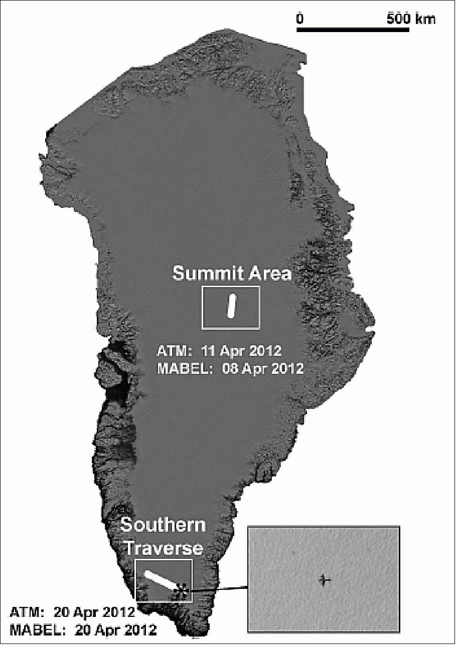
The NASA IceBridge ATM Level-2 Icessn Elevation, Slope, and Roughness (ILATM2) for April 11 and 20, 2012, were obtained from the National Snow and Ice Data Center (NSIDC). This is a resampled and smoothed elevation data set that provides four across-track elevations per timestamp every ~35 m along-track, which allowed for the trivial calculation of across-track slope. The total across-track span for this data set, for the flights used in this analysis, was approximately 150 m.
MABEL data (release 8) for April 8 and 20, 2012, were obtained from the NASA ICESat-2 website. Each data file contains 1 minute of data for every available beam. The data files contain photon arrival times resulting from reflected laser light (i.e., signal photons) and background photons due to sunlight (i.e., noise photons).
In order to discriminate coarse signal photons from noise photons and derive ice-sheet surface elevation, the team developed an algorithm based on histograms of the photon data. Evolving from techniques applied to other photon-counting lidars, such as the SIMPL (Slope Imaging Multi-polarization Photon-counting Lidar), a 0.125 s (~25 m; 625 shots) along-track segments of data was generated and the photon data at 10 m vertical resolution was histogrammed. Signal photons in four sequential steps were identified.
For direct comparison of the surveys, ATM tracks and MABEL beams were chosen to most closely mimic the 90 m spacing of the ICESat-2 beam geometry. ATM tracks 2 and 3 were used for this analysis because they have ground separation of ~85 m. Elevations from tracks 2 and 3 from the same along-track time were then used to calculate the ATM across-track slope. MABEL beam 6 (center of the array) and beam 5 (~85 m ground spacing from the center of the array) were chosen for analysis as they have an across-track ground separation similar to the ATM tracks used. To determine the MABEL across-track slope, signal photons from beams 5 and 6 were interpolated along track to a common time so that, similar to ATM, an across-track slope could be then calculated for each increment of along-track time. The across-track slopes for both ATM and MABEL were then compared.
MABEL beams have variable signal strengths; however, beams 5 and 6 are the most similar to the expected radiometry of the strong beams of ATLAS. The along-track data density differed within and between flights based on variables that affect reflectivity, including weather conditions, time of day, and sun-incidence angle. For the data used in this analysis, the full-rate along-track data density average for both beams was always greater than 4 signal photons/m. For the Southern Traverse flight, the along-track data densities were 3.4 and 3.9 signal photons per 70 cm for beams 5 and 6, respectively. For the Summit Area flight, data densities were 3.1 and 3.4 signal photons per 70 cm for beams 5 and 6, respectively.
A strong-beam/weak-beam pair will be used for ICESat-2 slope determination; the energy associated with the weak beam will be reduced by a factor of 4. Therefore, the expected number of signal photons per laser shot (every 70 cm along track) between the strong beam and the weak beam will also differ by a factor of 4. The current best estimates of expected signal photons per laser shot vary with season and surface type. Based on ICESat-2 engineering models, under similar conditions as the 2012 MABEL survey, the team expects ICESat-2 to record 8.5 and 2.1 signal photons every shot (or 70 cm along track) for the strong and weak beams, respectively. Thus, the MABEL full-rate data used in this analysis suggest data densities of 46% of the expected ICESat-2 data densities. MABEL engineers are currently working to increase signal strength to achieve the expected ICESat-2 data densities, which will facilitate more direct MABEL to ATLAS comparisons.
To further assess accurate ground characterization given the ICESat-2 planned configuration, all photons associated with one of the MABEL beams (beam 5) were subsampled by a factor of 4 and then reprocessed through the ground-finding algorithm, to simulate the expected radiometric relationship between the ATLAS strong and weak beams. After subsampling, the data densities were 0.9 and 0.8 signal photons per 70 cm for the Southern Traverse and Summit Area, respectively. To determine the MABEL across-track slope, the ground-signal photons from beam 6 and the subsampled ground-signal photons from beam 5 were again interpolated to a common time so that an across-track slope could be calculated as described above. Therefore, the beam with the fewest along-track samples (the weak beam, 5) limited the total number of samples that was used in the slope determination.
Antarctic Preparatory Campaign
In temperatures that can drop below -20º Fahrenheit (-29ºC), along a route occasionally blocked by wind-driven ice dunes, a hundred miles from any other people, a team led by two NASA scientists will survey an unexplored stretch of Antarctic ice. 87)
They’re packing extreme cold-weather gear and scientific instruments onto sleds pulled by two tank-like snow machines called PistenBullys, and on 21 Dec. 2017, they will begin their two- to three-week traverse in an arc around the South Pole.
The 470-mile (759 km) expedition in one of the most barren landscapes on Earth will ultimately provide the best assessment of the accuracy of data collected from space by ICESat-2 (Ice Cloud and land Elevation Satellite-2), set to launch in 2018. With a fast-firing laser instrument, ICESat-2 will measure the elevation of ice sheets and track change over time. Even small amounts of melt across areas as vast as Greenland or Antarctica can result in large amounts of meltwater contributing to sea level rise.
To help document this, ICESat-2's height change measurements will have a precision of less < 2.5 cm – ground-truthed, in part, with efforts like this Antarctic campaign. The team will collect precise GPS data of the elevation at 88 degrees south, where ICESat-2’s orbits converge, providing thousands of points where the survey measurements can be compared to satellite data.
“This traverse provides an extremely challenging and extremely cold way to assess the accuracy of the data,” said Kelly Brunt, ICESat-2’s calibration and validation lead at NASA/GSFC (Goddard Space Flight Center), and a research scientist at the University of Maryland. “ICESat-2’s datasets are going to tell us incredible things about how Earth’s ice is changing, and what that means for things like sea level rise.”
Brunt is leading the four-person campaign from the South Pole, along with ICESat-2’s deputy project scientist Tom Neumann. The NASA scientists will also be joined by a mechanic and a deep field mountaineer. The campaign to collect these key elevation measurements has been years in the making, with logistical help from the National Science Foundation’s U.S. Antarctic Program.
It will be a really cold road trip, Brunt said. They’ll wake up, make coffee (with beans, grounds and pour-over equipment chosen and packed with great care), turn on the snow machines and instruments, and start the day’s drive. The two PistenBullys will each tow a thick plastic sled, about 8 feet wide and 60 feet long. The sleds – kind of like extra-large Flexible Flyers, Neumann noted – will carry tents as well as food, equipment and extra fuel.
The whole trek is about 750 km. The team will leave the South Pole along an established traverse line between the southernmost station and McMurdo. Just after they reach 88º south, they will turn and follow the latitude line for about 186 miles. Then, they’ll turn back to the pole – creating a route like a misshapen piece of pie. At a pace of 50 to 72 km/day, it will take at least a couple weeks to complete.
“There’ll be times when it’s quiet and thoughtful, and there are going to be other times when you’re steering around the sastrugi – the sand dunes of the ice – when you’re not going to make a lot of kilometers on that day, but they’ll be hard fought,” Kelly Brunt said.
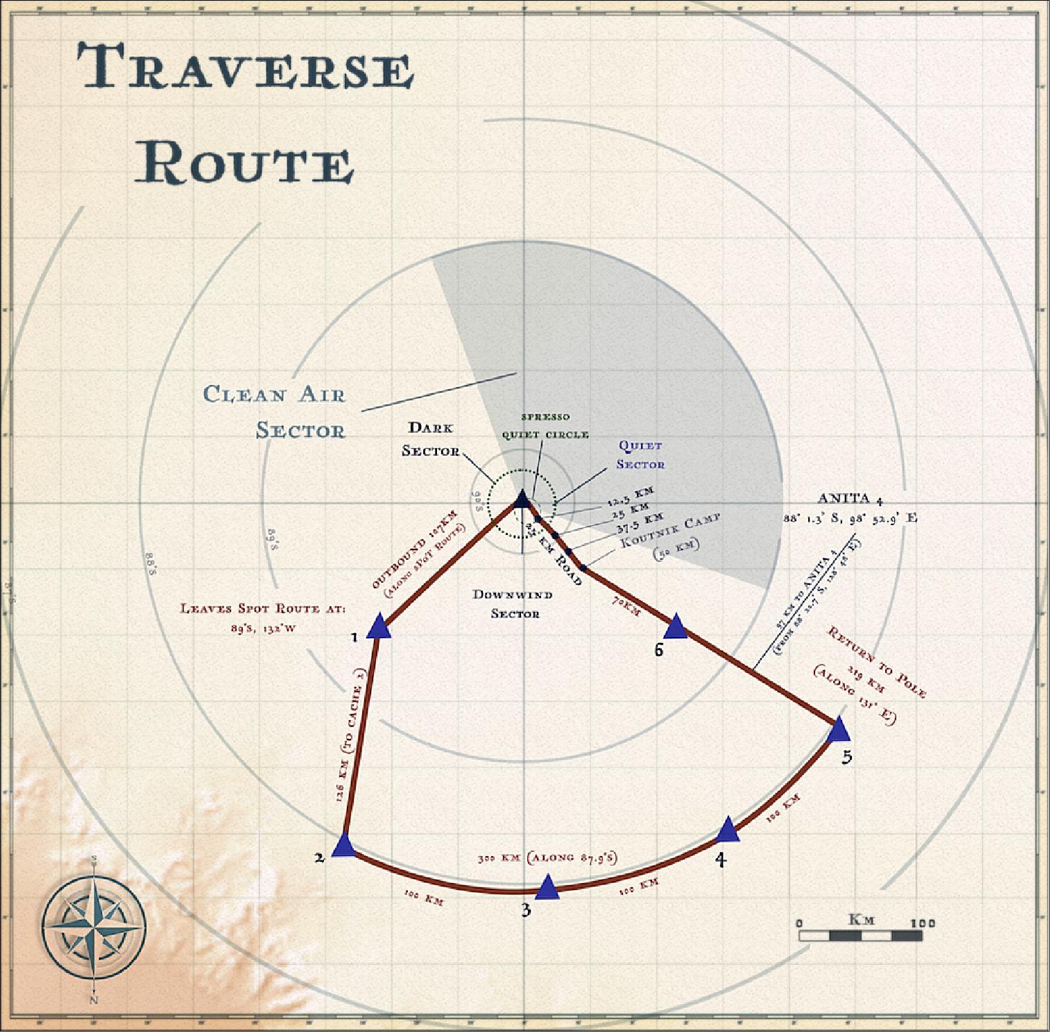
Crevasses are highly unlikely in this thick, slow-moving region of the Antarctic ice sheet, she said. The campaign’s deep field mountaineer will operate a ground penetrating radar that sticks out on a boom in front of the lead vehicle, looking for any gaps in the ice, but the primary safety concerns will be exposure to outside temperatures (-30ºC) and the altitude (about 3 km at South Pole).
The first few days at the South Pole station will be spent acclimatizing to the altitude, Neumann said, noting that the cold, dry air makes the environment even harsher. Once on the road, however, he plans to spend evenings out in the elements, digging holes.
“I’ll measure the density of the snow along the way,” he said. By shoveling out a three-foot-deep pit, he can see layers of snow that have built up over decades, some of which can be hard to dig past. “They’re not super dense, but they’re so old the grains of snow are bonded together like its cement.”
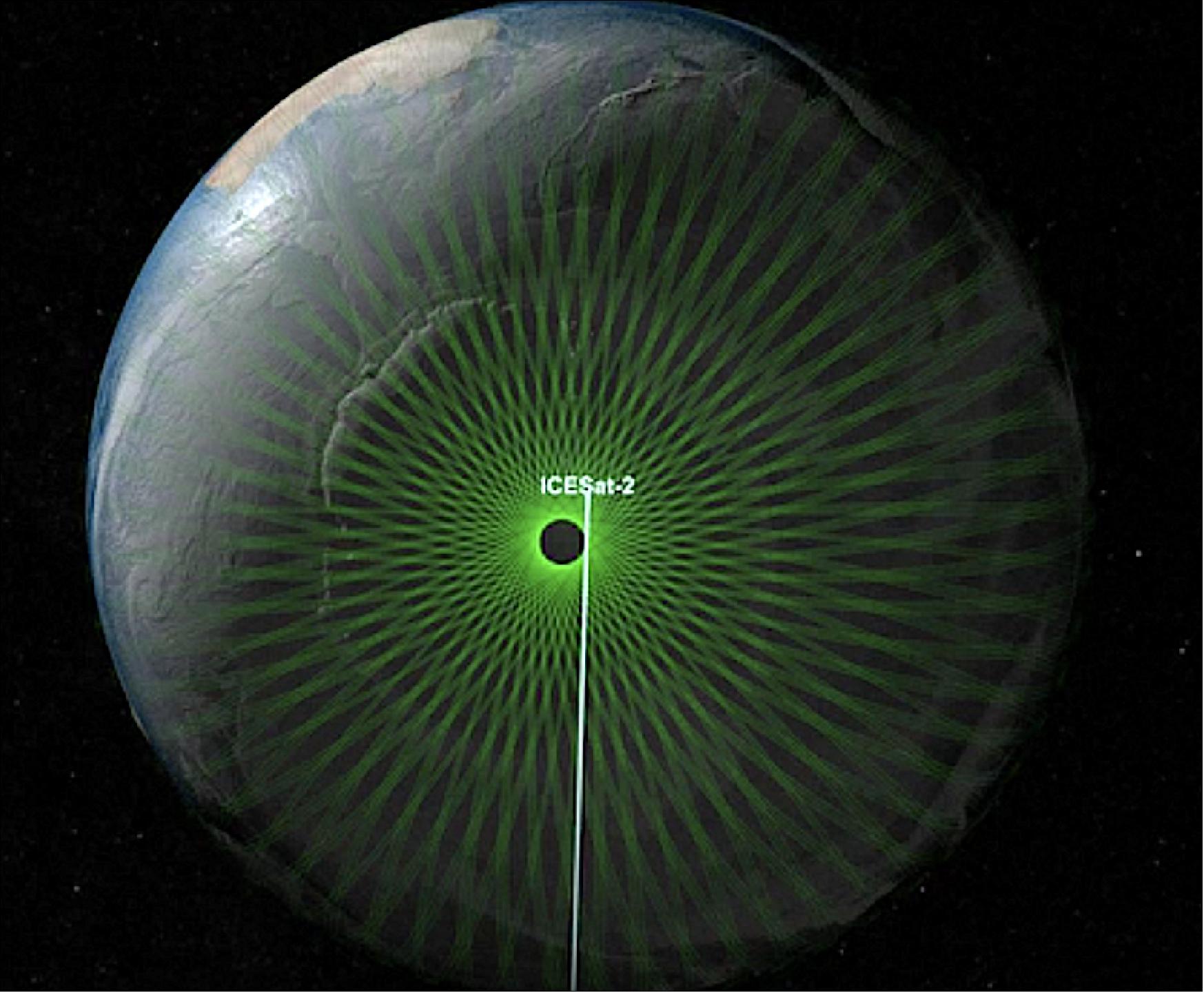
When ICESat-2 starts collecting elevation data, the snow density measurements and the data from the ground penetrating radar will help determine how much mass is lost when the ice sheet drops in elevation.
The 88-degree traverse is also an opportunity for Brunt and Neumann to play the odds. At three different sites along the route, they’ll set up a grid of nine reflector cubes, each no bigger than the tip of a pinkie finger. They’ll mark the precise latitude, longitude, and elevation of each cube.
Then, once ICESat-2 is up and running, they’ll wait. If one of the satellite’s six laser beams hits a cube, the mirrored material of the cube will reflect the laser light back at a much higher than normal intensity. Since they’ll know the exact location and elevation of the cube, they can check the accuracy of the satellite data even more precisely than with the traverse data.
“If you hit that tiny little point, you’ll know exactly where the laser hit on the ground,” Brunt said. “But hitting that point is both aiming and luck. It’s hard. But, by placing them at 88 degrees, where you have so many orbits crossing and so much data, it’s just a statistics game.”
After the traverse, the scientists will return to the United States, retracing their steps from the South Pole station, to McMurdo Station, to New Zealand and home. With them: hard drives full of data to help understand the accuracy of ICESat-2.

NASA Operation IceBridge Campaign in Antarctica 2017
This campaign is intended to be flown by NASA's P-3 aircraft, beginning in late October and ending in late November 2017. The mission, called Operation IceBridge, is in its ninth year of flights to map the snow and ice of Antarctica. The view from above provides a tremendous amount of information about the huge expanses of snow and ice around Earth’s polar regions and how they are changing. 89) 90)
Some flight lines are designed to map the ice laying atop the land, while others map the sea ice. On November 4, 2017, the IceBridge team flew its “Endurance West” mission, which specifically targets sea ice. The P3 crossed the northern tip of the Antarctic Peninsula, descended to a lower altitude, and then flew southward across the Weddell Sea. The path purposely follows a ground track of ICESat-2 —an ice-mapping satellite mission that is scheduled for launch in late 2018.
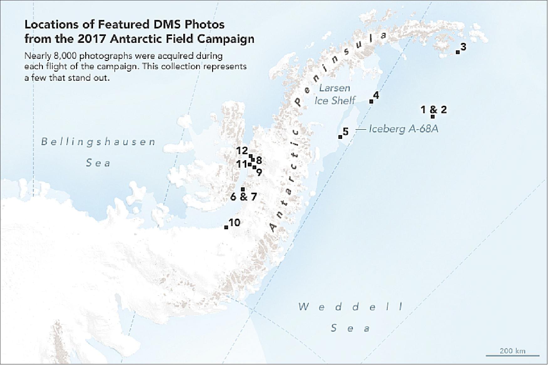
Images from that day show just how varied sea ice can appear. The first photograph, shot from the aircraft by IceBridge project scientist Nathan Kurtz, shows newly formed sea ice next to a snow-covered floe in the Weddell Sea. The second and third images, both acquired by the DMS (Digital Mapping System), show sea ice off the Antarctic Peninsula. Thicker ice is white, thinner ice is gray, and open water is black or navy.
Note: Only a few images, marked in Figure 79, are provided here.
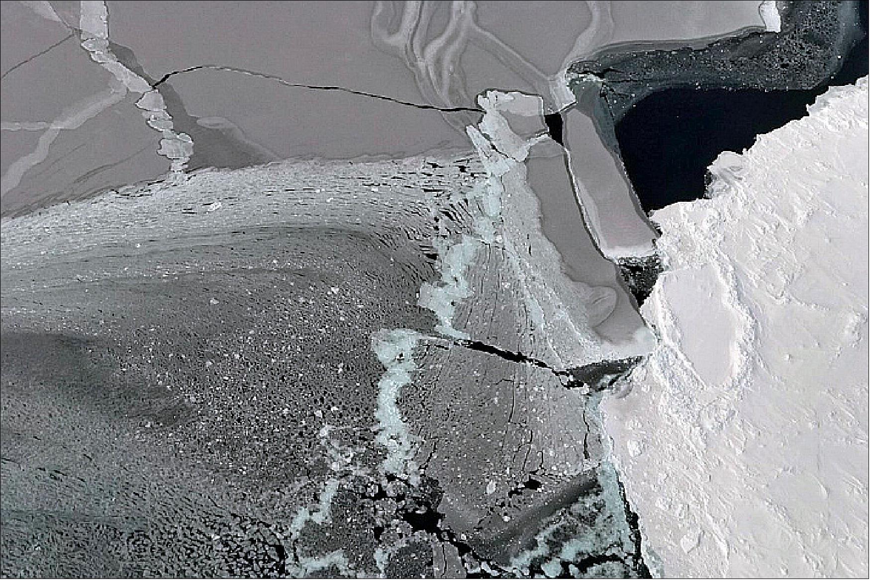
On November 12, 2017, IceBridge flew a high-priority mission over the Larsen C Ice Shelf. In July 2017, this region was significantly reshaped by the shedding of an iceberg the size of Delaware. For most of the four-hour survey, as the aircraft flew back-and-forth in parallel lines over the ice shelf, the landscape appeared flat and white. These new flight lines followed the ground tracks of the future ICESat-2, providing baseline measurements for the satellite to take over after it begins operations. This survey also increased the amount of Larsen C that has been observed with a gravimeter, an instrument that helps scientists map the bedrock below the ice shelf and the water, which radar and visual imagers cannot penetrate.
Visually, the landscape appeared more varied when the aircraft traced the edge of the ice shelf or soared over sea ice. These photographs show sea ice of various types as observed by the DMS during the November 12 flight.
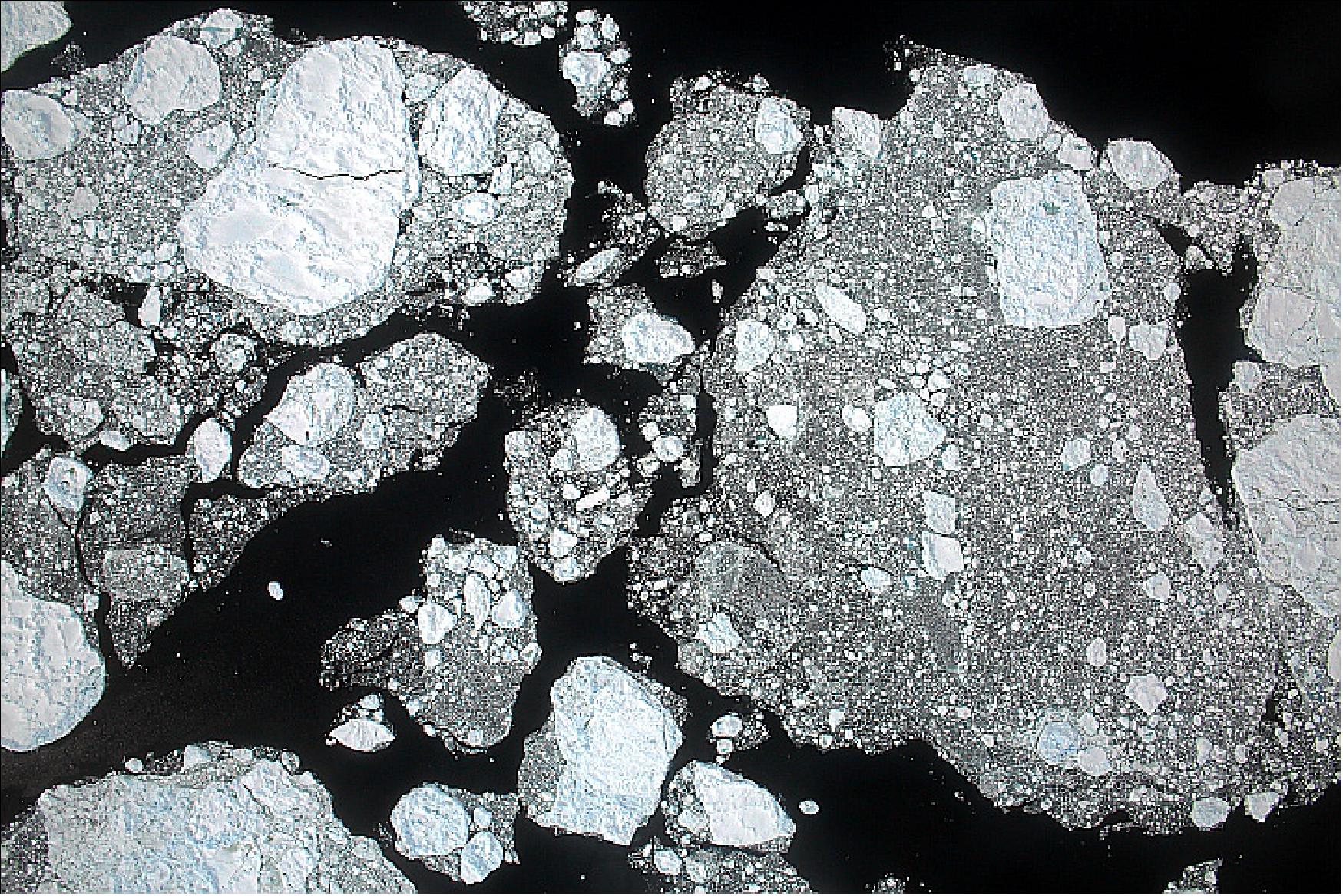
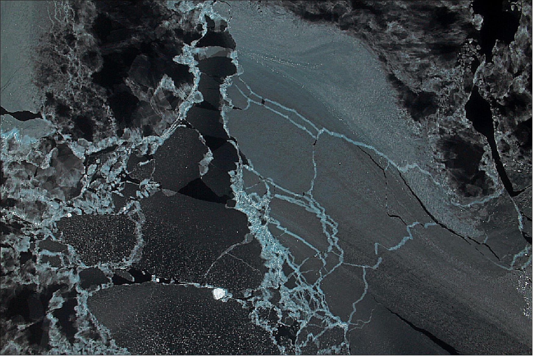
Fractures: During any given IceBridge flight, one can see areas of fractures and crevasses that attest to lumbering motion of huge slabs of ice. Its thickness on this part of the continent can vary dramatically, from no ice at all (barren bedrock) to more than a kilometer thick. The reason for the brittle appearance is similar to the phenomenon of river rapids, which become amplified as water flows through steep, narrow terrain. As ice flows through narrower areas and steeper bedrock, more fractures open up at the ice surface. But the flow of ice is so much slower than water, and fractures are often the only perceptible indication of movement. These images, acquired by the DMS on November 3, 2017, show cracks in the ice as observed while flying over the southern Antarctic Peninsula.
The image of Figure 83 shows a heavily crevassed glacier, about 13 miles long and 7 miles wide, flowing west from the Dyer Plateau to George VI Sound. The north side of this glacier merges with Meiklejohn Glacier.
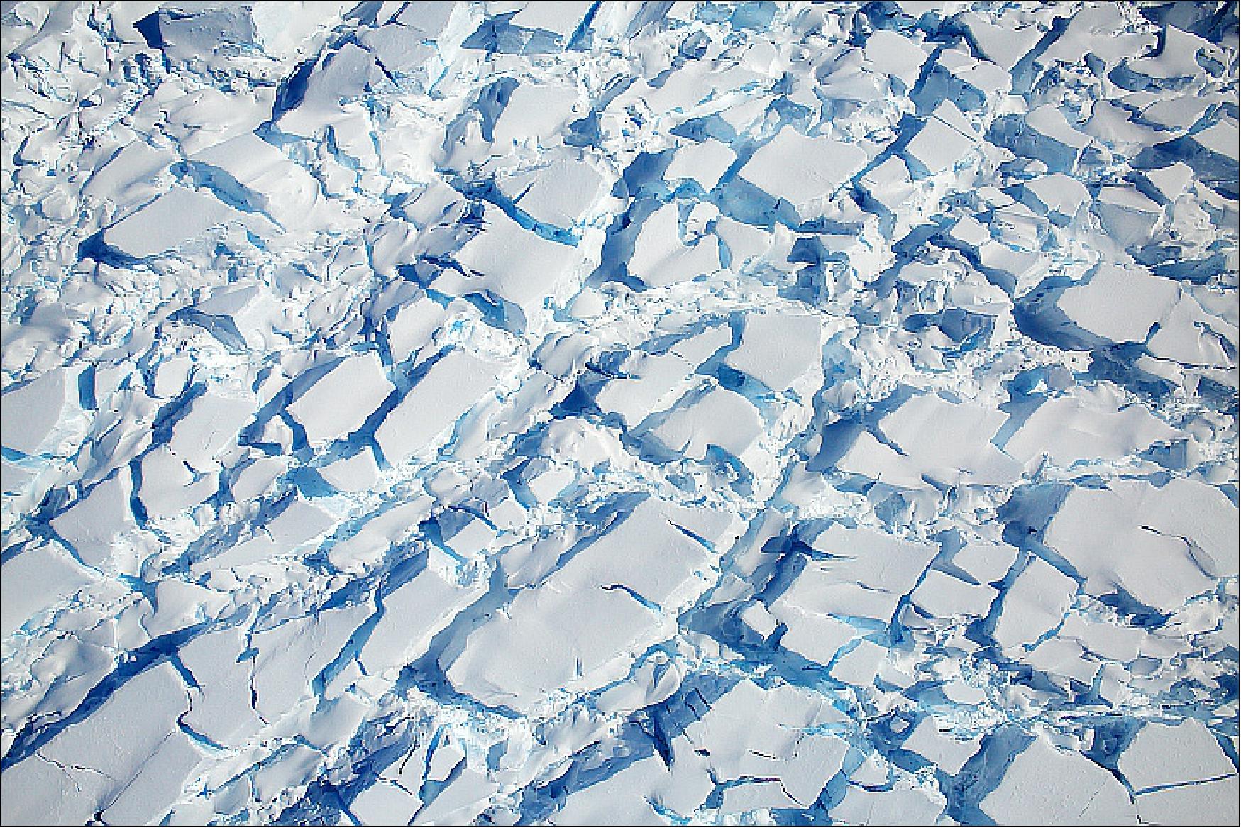
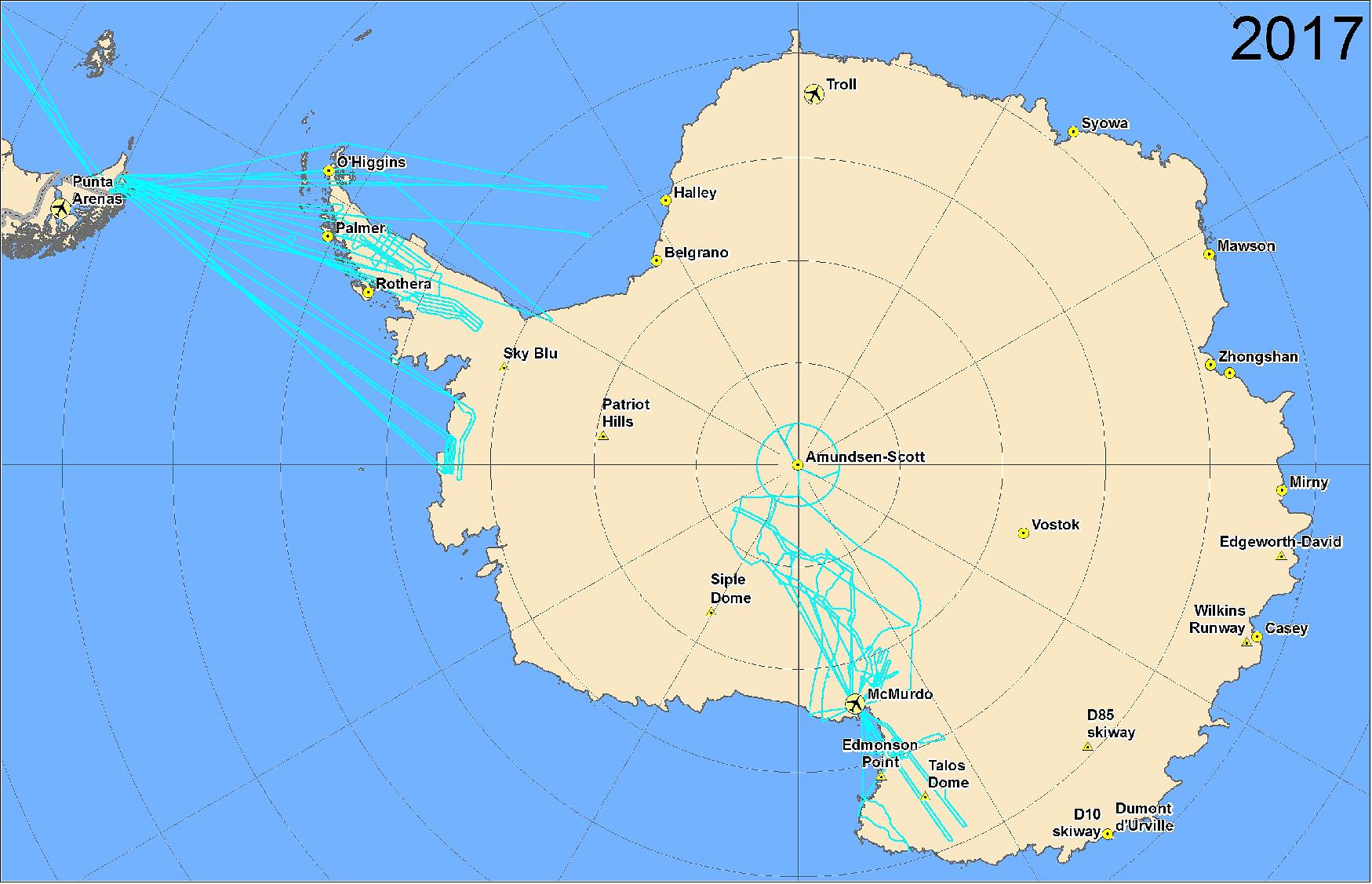
References
1) Waleed Abdalati, H. Jay Zwally, Robert Bindschadler, Bea Csatho, Sinead Louise Farrell, Helen Amanda Fricker, David Harding, Ronald Kwok, Michael Lefsky, Thorsten Markus, Allexander Marshak, Thomas Neumann, Stephen Palm, Bob Schutz, Ben Smith, James Spinhirne, Charles Webb, “The ICESat-2 Laser Altimetry Mission,” Proceedings of the IEEE. Vol 98, No. 5, May 2010. Pages 735-751., URL: http://icesat.gsfc.nasa.gov/icesat2/publications/pubs_2010/abdalati_et_al_2010.pdf
2) Douglas D. McLennan, “Ice, Clouds and Land Elevation (ICESat-2) Mission,” Proceedings of the SPIE Remote Sensing Conference, Toulouse, France, Vol. 7826, Sept. 20-23, 2010, paper: 7826-32, 'Sensors, Systems, and Next-Generation Satellites XIV,' edited by Roland Meynart, Steven P. Neeck, Haruhisa Shimoda, doi: 10.1117/12.865200
3) “ICESat-2,” NASA/GSFC, URL: http://icesat.gsfc.nasa.gov/icesat2/
4) David J. Harding, “NASA's Lidar measurements of the Earth's surface from space,” Proceedings of IGARSS (International Geoscience and Remote Sensing Symposium), Munich, Germany, July 22-27, 2012
5) Molly Brown, Mark Carroll, Vanessa Escobar, “ICESat-2 Applications Workshop Report, NASA Goddard Space Flight Center, April 12, 2012, URL: http://icesat.gsfc.nasa.gov/icesat2/applications/ICESat2_Applications_Workshop1_Report_final.pdf
6) Kelly M. Brunt, Sinéad L. Farrell, Vanessa M. Escobar, “ICESat-2: A next generation laser altimeter for space-borne determination of surface elevation,” 93rd American Meteorological Society Annual Meeting, Austin, TX, USA, Jan. 6-10, 2013, URL: https://ams.confex.com/ams/93Annual/webprogram/Handout/Paper224015/BruntAMS2013.pdf
7) http://icesat-2.gsfc.nasa.gov/
8) “Earth Science and Applications from Space,” NASA, NAS (National Academy of Sciences), URL: http://cce.nasa.gov/pdfs/ICESAT-II.pdf
9) Tom Newmann, Thorsten Markus, Matthew McGill, Kelly Brunt, Tony Martino, William Cook, “MABEL and the ICESat-2 Mission: Photon-counting Altimetry from Air and Space,” The Earth Observer, Sept.-Oct. 2012, Volume 24, Issue 5, pp: 4-8, URL: http://eospso.gsfc.nasa.gov/sites/default/files/eo_pdfs/Sept_Oct_2012_color_508.pdf
10) https://icesat-2.gsfc.nasa.gov/mission
11) S. Volz, “NASA Earth Sciience New Miissiion Concepts for the Future,” 5th SORCE Science Meeting, Santa Fee, NM, Feb. 7, 2008, URL: http://lasp.colorado.edu/sorce/news/2008ScienceMeeting/doc/Session4/S4_08_Volz.pdf
12) John Loiacono, ICESat-2 Progress Report for FY08 and FY09 Plans,” Feb. 11, 2009, URL: http://decadal.gsfc.nasa.gov/documents/03_ICESat_II.pdf
13) “Orbital Wins ICESat-2 Earth Science Satellite Program Contract,” Space Daily, Sept. 2, 2011, URL: http://www.spacedaily.com/reports/Orbital_Wins_ICESat_2_Earth_Science_Satellite_Program_Contract_999.html
14) “NASA Selects Contractor For Icesat-2 Spacecraft,” NASA, Aug. 31, 2011, URL: http://www.nasa.gov/home/hqnews/2011/aug/HQ_C11-037_ICESat2.html
15) “ICESat-2,”, Orbital ATK, URL: https://web.archive.org/web/20161025235444/https://www.orbitalatk.com/space-systems/science-national-security-satellites/science-environment-satellites/docs/ICESat-2.pdf
16) Kate Ramsayer, ”ICESat-2 Lasers Pass Final Ground Test,” NASA, 9 July 2018, URL: https://www.nasa.gov/feature/goddard/2018/icesat-2-lasers-pass-final-ground-test
17) ”Northrop Grumman Completes Orbital ATK Acquisition, Blake Larson Elected to Lead New Innovation Systems Sector,” Northrop Grumman News, 6 June 2018, URL: https://news.northropgrumman.com/news/releases/northrop-grumman-completes-orbital-atk-acquisition-blake-larson-elected-to-lead-new-innovation-systems-sector
18) Kate Ramsayer, ”NASA space laser completes 2,000-mile road trip,” Space Daily, 1 March 2018, URL: http://www.spacedaily.com/reports/NASA_Space_Laser_Completes_2000_mile_Road_Trip_999.html
19) Kate Ramsayer , Sara Blumberg, ”NASA's ICESat-2 Preps for Laser Tests,” NASA, Aug. 16, 2017, URL: https://www.nasa.gov/feature/goddard/2017/nasas-icesat-2-preps-for-laser-tests
20) Michael Freilich, ”ICESat-2 Technical Status Summary,” The National Academies of Sciences, Engineering, and ..., Sept. 1, 2016, URL: http://sites.nationalacademies.org/cs/groups/ssbsite/documents/webpage/ssb_174609.pdf
21) ”ICESat-2: Status Updates,” NASA, URL: http://icesat.gsfc.nasa.gov/icesat2/status.php
22) Kate Ramsayer, ”NASA tests ICESat-2's laser aim,” NASA, Dec. 10, 2015, URL: http://www.nasa.gov/feature/goddard/lasers-path-through-icesat-2
23) Kate Ramsayer, “NASA's ATLAS thermal testing: You're hot, then you're cold,” NASA, April 21, 2015, URL: http://phys.org/news/2015-04-nasa-atlas-thermal-youre-hot.html
24) “NASA lining up ICESat-2's laser-catching telescope,” NASA, Nov. 3, 2014, URL: http://phys.org/news/2014-11-nasa-lining-icesat-laser-catching-telescope.html#inlRlv
25) Dan Leone, “Paying for ICESat-2 Overruns Delays International Earth Science Launches,” Space News, Sept. 1, 2014, URL: http://spacenews.com/41729paying-for-icesat-2-overruns-delays-international-earth-science-launches/
26) Stephen Clark, “Over-budget ICESat 2 mission under review,” Spaceflight Now, Dec. 10, 2013, URL: http://spaceflightnow.com/news/n1312/10icesat2/#.U5lV4Ha4Ri0
27) ”NASA, ULA Launch Mission to Track Earth's Changing Ice,” NASA Release 18-078, 15 September 2018, URL: https://www.nasa.gov/press-release/nasa-ula-launch-mission-to-track-earths-changing-ice
28) ”2018: A Big Year for NASA's Launch Services Program,” NASA, 1 Feb. 2018, URL: https://www.nasa.gov/feature/2018-a-big-year-for-nasas-launch-services-program
29) ”About ICESat-2,” NASA, 2017, URL: [web source no longer available]
30) ”ELFIN,” UCLA, 9 March 2018, URL: http://elfin.igpp.ucla.edu/
31) Kate Ramsayer, ”NASA Approves Continuation of ICESat-2 After 3+ Years of Big Results,” NASA, 28 June 2022, URL: https://www.nasa.gov/goddard/2022/nasa-approves-continuation-of-icesat-2-after-3-years-of-big-results
32) ”NASA Awards Mission Operations Center Support Contract,” NASA Contract Release, 10 February 2022, URL: https://www.nasa.gov/press-release/nasa-awards-mission-operations-center-support-contract
33) Roberto Molar Candanosa, Ellen Gray, ”NASA Space Lasers Map Meltwater Lakes in Antarctica With Striking Precision,” NASA Feature, 7 July 2021, URL: https://www.nasa.gov/feature/goddard/2021/nasa-space-lasers-map-meltwater-lakes-in-antarctica-with-striking-precision
34) M. R. Siegfried, H. A. Fricker, ”Illuminating active subglacial lake processes with ICESat-2 laser altimetry,” Geophysical Research Letters, Firts published: 07 July 2021, https://doi.org/10.1029/2020GL091089
35) ”Sizing Up a Tabular Iceberg,” NASA Earth Observatory, 3 June 2021, URL: https://earthobservatory.nasa.gov/images/148388/sizing-up-a-tabular-iceberg
36) ”Sounding the Seafloor with Light,” NASA Earth Observatory, Image of the Day for 30 April 2021, URL: https://earthobservatory.nasa.gov/images/148246/sounding-the-seafloor-with-light
37) N. Thomas, A. P. Pertiwi, D. Traganos, D. Lagomasino, D. Poursanidis, S. Moreno, L. Fatoyinbo, ”Space‐Borne Cloud‐Native Satellite‐Derived Bathymetry (SDB) Models Using ICESat‐2 And Sentinel‐2,” Geophysical Research Letters, Volume48, Issue6, 28 March 2021, e2020GL092170, https://doi.org/10.1029/2020GL092170, URL: https://agupubs.onlinelibrary.wiley.com/doi/epdf/10.1029/2020GL092170
38) ”Sizing Up Remote Lakes,” NASA Earth Observatory, Image of the Day for 27 April 2021, URL: https://earthobservatory.nasa.gov/images/148230/sizing-up-remote-lakes
39) Kate Ramsayer, ”NASA Scientists Complete 1st Global Survey of Freshwater Fluctuation,” NASA Feature, 3 March 2021, URL: https://www.nasa.gov/feature/goddard/2021/nasa-scientists-complete-first-global-survey-of-freshwater-fluctuation
40) Sarah W. Cooley, Jonathan C. Ryan & Laurence C. Smith, ”Human alteration of global surface water storage variability,” Nature, Volume 591, pp:78-81, Published: 03 March 2021, https://doi.org/10.1038/s41586-021-03262-3
41) Kate Ramsayer, ”Beyond Ice: NASA’s ICESat-2 Shows Hidden Talents,” NASA Feature, 9 December 2020, URL: https://www.nasa.gov/feature/goddard/2020/beyond-ice-nasa-s-icesat-2-shows-hidden-talents
42) ”Taking a Measure of Sea Level Rise: Ice Height,” NASA Earth Observatory, Image of the Day for 9 November 2020, URL: https://earthobservatory.nasa.gov/images/147438/taking-a-measure-of-sea-level-rise-ice-height?src=eoa-iotd
43) ”TCarta develops AI-based commercial bathymetric mapping technologies,” Space Daily, 27 October 2020, URL: https://www.spacedaily.com/reports/TCarta_develops_AI_based_commercial_bathymetric_mapping_technologies_999.html
44) ”Mapping Shallow Seafloors,” NASA Earth Observatory, Image of the Day for 29 September 2020, URL: https://earthobservatory.nasa.gov/images/147338/mapping-shallow-seafloors
45) ”Cracking Icy Secrets of New Penguin Colonies,” NASA Earth Observatory, Image of the Day for24 September 2020, URL: https://earthobservatory.nasa.gov/images/147310/cracking-icy-secrets-of-new-penguin-colonies
46) Aries Keck, ”Pinpointing Tropical Forests with High Ecological 'Quality',” NASA Earth, 25 August 2020, URL: https://www.nasa.gov/feature/pinpointing-tropical-forests-with-high-ecological-quality
47) Andrew J. Hansen, Patrick Burns, Jamison Ervin, Scott J. Goetz, Matthew Hansen, Oscar Venter, James E. M. Watson, Patrick A. Jantz, Anne L. S. Virnig, Kevin Barnett, Rajeev Pillay, Scott Atkinson, Christina Supples, Susana Rodríguez-Buritica & Dolors Armenteras, ”A policy-driven framework for conserving the best of Earth’s remaining moist tropical forests,” Nature Ecology & Evolution, Volume 612, Published: 10 August 2020, https://doi.org/10.1038/s41559-020-1274-7
48) Kate Ramsayer, ”Syncing NASA Laser, ESA Radar for a New Look at Sea Ice,” NASA/GSFC, 16 July 2020, URL: https://www.nasa.gov/feature/goddard/2020/syncing-nasa-laser-esa-radar-for-a-new-look-at-sea-ice
49) ”Mapping Snow on Arctic Sea Ice,” NASA Earth Observatory, Image of the Day for 27 May 2020, URL: https://earthobservatory.nasa.gov/images/146758/mapping-snow-on-arctic-sea-ice
50) R. Kwok, S. Kacimi, M.A. Webster, N. T. Kurtz, A. A. Petty, ”Arctic Snow Depth and Sea Ice Thickness From ICESat‐2 and CryoSat‐2 Freeboards: A First Examination,” JGR (Journal of Geophysical Research) Oceans, Volume125, Issue3, 10 March 2020, e2019JC016008, https://doi.org/10.1029/2019JC016008
51) Kate Ramsayer, ”NASA’s ICESat-2 Measures Arctic Ocean’s Sea Ice Thickness, Snow Cover,” NASA Feature, 14 May 2020, URL: https://www.nasa.gov/feature/goddard/2020/icesat-2-measures-arctic-sea-ice-thickness-snow-cover
52) Alek A. Petty, Nathan T. Kurtz, Ron Kwok,Thorsten Markus, Thomas A. Neumann, ”Winter Arctic Sea Ice Thickness From ICESat‐2 Freeboards,” JGR (Journal of Geographical Research): Oceans, Volume125, Issue5, Published: 15 May 2020, e2019JC015764, https://doi.org/10.1029/2019JC015764
53) R. Kwok, S. Kacimi, M.A. Webster, N. T. Kurtz, A. A. Petty, ”Arctic Snow Depth and Sea Ice Thickness From ICESat‐2 and CryoSat‐2 Freeboards: A First Examination,” JGR Oceans, Volume 125, Issue 3, Published: 10 March 2020, e2019JC016008, https://doi.org/10.1029/2019JC016008
54) ”NASA Space Laser Missions Map 16 Years of Ice Sheet Loss,” NASA/JPL News Release 2020-086 , 30 April 2020, URL: https://www.jpl.nasa.gov/news/news.php?release=2020-086
55) Ben Smith, Helen A. Fricker, Alex S. Gardner, Brooke Medley, Johan Nilsson, Fernando S. Paolo, Nicholas Holschuh, Susheel Adusumilli, Kelly Brunt, Bea Csatho, Kaitlin Harbeck, Thorsten Markus, Thomas Neumann, Matthew R. Siegfried, H. Jay Zwally, ”Pervasive ice sheet mass loss reflects competing ocean and atmosphere processes,” Science, 30 Apr 2020: eaaz5845, https://doi.org/10.1126/science.aaz5845
56) Jessica Merzforf, ”NASA's Operation IceBridge Completes Eleven Years of Polar Surveys,” 13 December 2019, URL: https://climate.nasa.gov/news/2941/nasas-operation-icebridge-completes-eleven-years-of-polar-surveys/
57) ”A Transylvanian Transect for Halloween,” NASA Earth Observatory, Image of the Day for 1 November 2019, URL: https://earthobservatory.nasa.gov/images/145807/a-transylvanian-transect-for-halloween?src=eoa-iotd
58) ”Lake Mead by the Seasons,” NASA Earth Observatory, 18 October 2019, URL: https://earthobservatory.nasa.gov/images/145743/lake-mead-by-the-seasons
59) ”ICESat-2 Celebrates One Year for Photon Phriday,” NASA, 16 September 2019, URL: https://www.youtube.com/watch?v=t3MWfuaDAqc&feature=youtu.be
60) ”The Ups and Downs of Crater Lake,” NASA Earth Observatory, Image of the Day for 29 July 2019, URL: https://earthobservatory.nasa.gov/images/145370/the-ups-and-downs-of-crater-lake
61) ”Flowing Antarctic Ice Mapped 10 Times More Accurately,” NASA/JPL News, 29 July 2019, URL: https://www.jpl.nasa.gov/news/news.php?release=2019-153
62) J. Mouginot, E. Rignot, B. Scheuchl, ”Continent‐wide, interferometric SAR phase, mapping of Antarctic ice velocity,” Geophysical Research Letters, 29 July 2019, https://doi.org/10.1029/2019GL083826
63) ”UCI, JPL glaciologists unveil most precise map ever of Antarctic ice velocity,” UCI News, 29 July 2019, URL: https://news.uci.edu/2019/07/29/uci-jpl-glaciologists-unveil-most-precise-map-ever-of-antarctic-ice-velocity/
64) Kate Ramsayer, Sara Blumberg, ”First ICESat-2 Global Data Released: Ice, Forests and More,” NASA, 28 May 2019, URL: https://www.nasa.gov/feature/goddard/2019/icesat-2-global-height-data-available-to-public
65) ”ICESat-2 Sees the Trees in Mexico,” NASA Earth Observatory, Image of the day for 29 January 2019, URL: https://earthobservatory.nasa.gov/images/144450/icesat-2-sees-the-trees-in-mexico
66) ”Taking Measure of Antarctic Terrain,” NASA Earth Observatory, Image of the day for 12 December 2018, URL: https://earthobservatory.nasa.gov/images/144367/taking-measure-of-antarctic-terrain
67) Kate Ramsayer, Sara Blumberg,”ICESat-2 Reveals Profile of Ice Sheets, Sea Ice, Forests,” NASA, 11 December 2018, URL: https://www.nasa.gov/feature/goddard/2018/icesat-2-reveals-profile-of-ice-sheets-sea-ice-forests
68) Kate Ramsayer, ”ICESat-2 Laser Fires for 1st Time, Measures Antarctic Height,” NASA, 3 October 2018, URL: https://www.nasa.gov/feature/goddard/icesat-2-laser-fires-for-1st-time-measures-antarctic-height
69) Sabrina Delgado Arias, Molly Brown, Steve Palm, Yuekui Yang, Thomas Neumann, ”NASA Missions Working Together for Improved Atmospheric Data: ICESat-2 Convenes Joint Atmospheric Tutorial,” The Earth Observer, September - October 2017, Volume 29, Issue 5, pp: 20-30, URL: https://eospso.nasa.gov/sites/default/files/eo_pdfs/Sept_Oct_%202017_color.pdf
70) Julia M. Ruth, Sinead L. Farrell, Kelly M. Brunt, “Assessment of Arctic sea ice freeboard from photon-counting laser altimetry: Pre-launch activities for NASA’s ICESat-2 Mission,” URL: http://www.whoi.edu/fileserver.do?id=169388&pt=2&p=180851
71) Nicholas A. Forfinski-Sarkozi, Christopher E. Parrish, ”Analysis of MABEL Bathymetry in Keweenaw Bay and Implications for ICESat-2 ATLAS,” Remote Sensing, Vol. 8, 2016, doi:10.3390/rs8090772, URL: http://www.mdpi.com/2072-4292/8/9/772/pdf
72) Anthony W. Yu, Mark A. Stephen, Steve X. Li, George B. Shaw, Antonios Seas, Edward Dowdye, Elisavet Troupaki, Peter Liiva, Demetrios Poulios, Kathy Mascetti, “Space Laser Transmitter Development for ICESat-2 Mission,” Proceedings of SPIE, Vol. 7578, LASE 2010, San Francisco, CA, USA, Feb. 15-18, 2010, 'Solid State Lasers XIX: Technology and Devices,' edited by W. Andrew Clarkson, doi: 10.1117/12.843342, URL: http://icesat.gsfc.nasa.gov/icesat2/publications/pubs_2010/Yu_et_al_2010.pdf
73) “Instrument: ATLAS,” WMO, 2012, URL: http://www.wmo-sat.info/oscar/instruments/view/51
74) Douglas D. McLennan, Thorsten Markus, Thomas Neumann, “ URL: http://www.scribd.com/doc/76177455/ICESat-2-ND-Presentation-4-18-11
75) Charon Birkett, T. Markus, T. Neumann, “The ICESat‐2 Mission - Laser altimetry of ice, clouds and land elevation ....and also ocean, coastal, and continental waters,” OSTM SWT (Science Working Team), San Diego, CA, USA, October 19-21, 2011, URL: http://www.aviso.oceanobs.com/fileadmin/documents/OSTST/2011/oral/03_Friday/Plenary/New%20Frontiers/07%20Birkett.ICESat2.pdf
76) Douglas D. McLennan, Thorsten Markus, Thomas Neumann, “The Vital Role of ICESat Data Products,” 2011, URL: http://media.aero.und.edu/space.edu/documents/2011_0418_McLennan_The_Vital_Role_of_ICESat_Data_Products.ppt
77) Kate Ramsayer, “How NASA Builds a Space Laser,” NASA, June 3, 2014, URL: http://www.nasa.gov/content/goddard/how-nasa-builds-a-space-laser/#.U5XcfS-7mwQ
78) Mahsa S. Moussavi, Waleed Abdalati, Ted Scambos, Amy Neuenschwander, ”Applicability of an automatic surface detection approach to micro-pulse photon-counting lidar altimetry data: implications for canopy height retrieval from future ICESat-2 data,” International Journal of Remote Sensing Vol. 35 , Issue 13,2014, pp: 5263-5279
79) M. Jasinski, T. Neumann, “The ICESat‐2 Mission: Objectives, concept, and opportunities for snow,” NASA Snow Remote Sensing Workshop, Boulder, CO, USA, Aug. 14-16, 2013, URL: http://nasasnowremotesensing.gi.alaska.edu/sites/default/files/Jasinski.pdf
80) Kate Ramsayer, “A Laser Beam’s Path Through NASA's ICESat-2,” NASA, June 30, 2015, URL: http://www.nasa.gov/feature/goddard/lasers-path-through-icesat-2
81) Nicholas Sawruk, Patrick Burns, Ryan Edwards, Viatcheslav Litvinovitch, Floyd Hovis, ”Flight laser transmitter development for NASA ice topography ICESat-2 space mission,” Proceedings of IGARSS (International Geoscience and Remote Sensing Symposium), Valencia, Spain, July 23-27, 2018
82) Vanessa Escobar, Sabrina Delgado Arias, Pam Posey, Thomas, Neumann, “Improving Operational Awareness Through ICESat-2 Applications Workshops: Cross-Mission Development,” The Earth Observer, May-June 2014, Volume 26, Issue 3, pp: 15-22, URL: http://eospso.gsfc.nasa.gov/earthobserver/may-jun-2014
83) ”2 Rectangular Icebergs Spotted on NASA IceBridge Flight,” NASA, 23 October 2018, URL: https://www.nasa.gov/image-feature/goddard/2018/2-rectangular-icebergs-spotted-on-nasa-icebridge-flight
84) Maria-José Viñas, ”Operation IceBridge, ICESat-2 Join Forces To Survey Antarctica,” NASA, 12 October 2018, URL: https://www.nasa.gov/feature/goddard/2018/operation-icebridge-icesat-2-join-forces-to-survey-antarctica
85) Kelly M. Brunt, Thomas A. Neumann, Jason M. Amundson, Jeffrey L. Kavanaugh, Mahsa S. Moussavi, Kaitlin M. Walsh, William B. Cook, Thorsten Markus, ”MABEL photon-counting laser altimetry data in Alaska for ICESat-2 simulations and development,” The Cryosphere, Vol. 10, pp:1707–1719, August 2016, doi:10.5194/tc-10-1707-2016, URL: http://www.the-cryosphere.net/10/1707/2016/tc-10-1707-2016.pdf
86) Kelly M. Brunt, Thomas A. Neumann, Kaitlin M. Walsh, Thorsten Markus, “Determination of Local Slope on the Greenland Ice Sheet Using a Multibeam Photon-Counting Lidar in Preparation for the ICESat-2 Mission,” IEEE Geoscience and Remote Sensing Letters, Vol. 11, No 5, May 2014, pp: 935-939, URL of abstract: http://ieeexplore.ieee.org/document/6623082/
87) Kate Ramsayer , ”NASA Scientists Embark on Extreme Antarctic Trek,” NASA, 14 December 2017, URL: https://www.nasa.gov/feature/goddard/2017/a-nasa-road-trip-at-the-bottom-of-the-world
88) ”Archive for ‘ICESat-2 Antarctic Traverse’,” NASA Earth Observatory, 12 Dec. 2017, URL: https://earthobservatory.nasa.gov/blogs/fromthefield/category/icesat-2-antarctic-traverse/
89) Kathryn Hansen, ”Antarctica from Above: Flying for Science, Finding Beauty,” NASA Earth Observatory, 11 Jan. 2018, URL: https://earthobservatory.nasa.gov/Features/OperationIceBridge/?src=features-hp&eocn=home&eoci=feature
90) John Sonntag, ”Fall 2017 IceBridge P-3 Flight Plans,” 29 September 2017 Draft, URL: https://icebridge.gsfc.nasa.gov/wp-content/uploads/2017/01/flightplans_basler_20170929.pdf
91)
”NASA Operation IceBridge - Antarctic -2017,” URL: https://icebridge.gsfc.nasa.gov/?page_id=1772
The information compiled and edited in this article was provided by Herbert J. Kramer from his documentation of: ”Observation of the Earth and Its Environment: Survey of Missions and Sensors” (Springer Verlag) as well as many other sources after the publication of the 4th edition in 2002. - Comments and corrections to this article are always welcome for further updates (eoportal@symbios.space).
Spacecraft Launch Mission Status Sensor Complement Ground Segment Preparatory Campaigns References Back to top