GCOM-W (Global Change Observation Mission - Water)
EO
JAXA
Atmosphere
Ocean
Global Change Observation MIssion (GCOM) is a two-satllite constellation mission to monitor changes in Earth’s environment, managed by the Japan Aerospace Exploration Agency (JAXA). GCOM satellites track geophysical properties such as precipitation patterns and atmospheric aerosol composition in order to aid scientists with climate change prediction and water management. The first satellite in the constellation, GCOM-W1 (water specialising), was launched in May 2012 and second, GCOM-C1 (climate change specialising), was launched in December 2017.
Quick facts
Overview
| Mission type | EO |
| Agency | JAXA |
| Mission status | Operational (extended) |
| Launch date | 17 May 2012 |
| Measurement domain | Atmosphere, Ocean, Land, Snow & Ice |
| Measurement category | Cloud type, amount and cloud top temperature, Liquid water and precipitation rate, Cloud particle properties and profile, Ocean colour/biology, Aerosols, Multi-purpose imagery (ocean), Multi-purpose imagery (land), Surface temperature (land), Vegetation, Albedo and reflectance, Surface temperature (ocean), Atmospheric Humidity Fields, Sea ice cover, edge and thickness, Soil moisture, Snow cover, edge and depth, Ocean surface winds, Inland Waters |
| Measurement detailed | Cloud top height, Ocean imagery and water leaving spectral radiance, Ocean chlorophyll concentration, Cloud cover, Cloud optical depth, Precipitation intensity at the surface (liquid or solid), Aerosol optical depth (column/profile), Cloud type, Color dissolved organic matter (CDOM), Cloud liquid water (column/profile), Land surface imagery, Vegetation type, Earth surface albedo, Leaf Area Index (LAI), Atmospheric specific humidity (column/profile), Land surface temperature, Sea surface temperature, Ocean suspended sediment concentration, Sea-ice cover, Snow cover, Soil moisture at the surface, Wind speed over sea surface (horizontal), Cloud top temperature, Normalized Differential Vegetation Index (NDVI), Snow water equivalent, Photosynthetically Active Radiation (PAR), Fraction of Absorbed PAR (FAPAR), Snow Grain Size, Fire radiative power, Snow surface temperature, Lake Surface Temperature, Sea-ice surface temperature |
| Instruments | SGLI, AMSR2 |
| Instrument type | Imaging multi-spectral radiometers (vis/IR), Imaging multi-spectral radiometers (passive microwave) |
| CEOS EO Handbook | See GCOM-W (Global Change Observation Mission - Water) summary |
Summary
Mission Capabilities
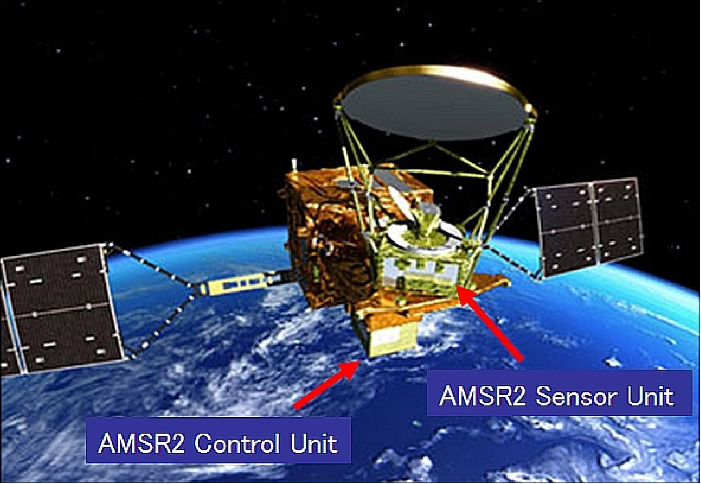
The primary instrument onboard GCOM-W1 is the Advanced Microwave Scanning Radiometer 2 (AMSR2). AMRS2 achieves measurements of Sea Surface Temperature (SST), Soil Moisture (SMD), Sea Surface Wind Speed (SSWS) and Sea Ice Concentration (SIC). The radiometer records multispectral microwave emissions from water-containing surface environments such as the ocean, sea ice and land. The data products are subsequently used by scientists to better understand the water cycle.
The primary instrument onboard GCOM-C1 is the Second Generation Global Imager (SGLI). SGLI is a multi-band optical radiometer consisting of two sensors SGLI-VNR - (Visible and Near Infrared Radiometer) and GLRI-IRS (Infrared Scanning Radiometer). SGLI collects data pertaining to the carbon cycle and atmospheric radiation budget. The VNR sensor’s polarimetry function is specifically optimised for detection of aerosol particle size, allowing for the corresponding aerosol source to be inferred.
Performance Specifications
ASMR2 employs a disc aperture design, with a nominal diameter of 2.0 m. This disc is rotated at a frequency of 0.66 Hz and scans with a swath width 1450 km. There are six imaging channels, with central frequencies ranging from 7.3 GHz to 89.0 GHz, each of which samples over a spatial interval of 10 km. SGLI samples over 19 channels, with central wavelength varying from the VNR spectral region (380 nm) up to the thermal infrared (TIR) region (12.0 μm). Spatial resolution is channel dependent but the finest resolution is 250 m and the most coarse is 1000 m.
Each satellite follows a Sun synchronous sub-recurrent orbit with GCOM-W travelling at an altitude of 699.6 km and GCOM-C1 slightly higher, at 798 km. Both satellites operate at approximately the same inclination of 98º.
Space and Hardware Components
JAXA have selected mid-sized satellites for the GCOM series, each with a design life of five years. GCOM-W1 is three-axis stabilised and the satellite attitude is controlled by four reaction wheels. The Electrical Power Subsystem (EPS) provides a power output of 4.05 kW. S-band radio frequency (RF) is used for Telecommunication, Telemetry and Control (TT&C) and the payload downlink is conducted over the X-band, at a data rate of 20 Mbit/s. Real-time observation data is transmitted to Japanese ground stations in Katsuura and Saitama.
GCOM-W (Global Change Observation Mission - Water)
GCOM-W1 Launch Mission Status Sensor Complement Ground Segment References
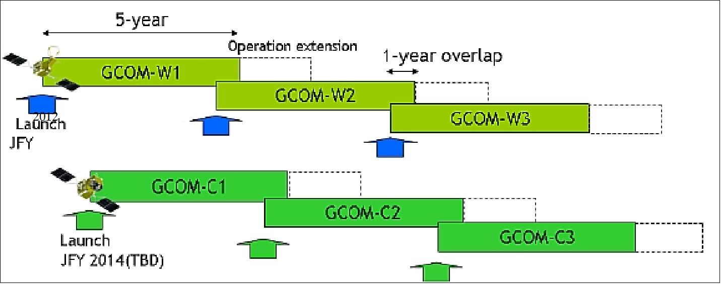
GCOM is a JAXA (Japan Aerospace Exploration Agency) observation program consisting of a constellation of two medium-sized spacecraft with the provisional names of GCOM-W and GCOM-C. GCOM is seen as a follow-up program to ADEOS.-II (launch Dec. 14, 2002) with the overall objective to contribute to global change research through long-term (> 10 years) sustained observations with corresponding data sets. Three consecutive constellations of spacecraft are being planned, representing in particular the long-term Japanese contribution to the GEOSS (Global Earth Observation System of Systems) initiative. The prime goal of GEOSS is to achieve comprehensive, coordinated and sustained observations of the Earth environment. 1) 2) 3) 4) 5) 6) 7) 8) 9) 10) 11) 12) 13)
The mission of GCOM is to achieve the following objectives:
• The primary goal of GCOM-W, a sea surface observation mission, is to contribute to observations related to global water and energy circulation. The payload consists of an AMSR2 (Advanced Microwave Scanning Radiometer-2) instrument.
Note: The AMSR instrument was flown on ADEOS-II mission (Dec. 14, 2002 to Oct. 25, 2003 - a power failure accident ended ADEOS-II) of JAXA, and the AMSR-E (for EOS) instrument is being flown on the Aqua mission of NASA (launch May 2002).
• The primary goal of the GCOM-C mission is to contribute to surface and atmospheric measurements related to the climate change with emphasis on the carbon cycle and the radiation budget. The payload consists of a second-generation GLI (SGLI) instrument.
The GCOM series will be maintained toward the final mission goal which should be accomplished by the end of 13 year observations, processing and analysis and application research period. The GCOM program calls for the following goals:
• The establishment of long-term observation system for the global carbon cycle and radiation budget, integrated with other earth observation systems.
• Contribution to numerical climate models (driving force, outputs comparison, and parameter tuning).
• Contribution to operational use (weather forecast, monitoring of meteorological disaster, fishery..).
• Enhancement of new satellite data usability.
GCOM is expected to make the following achievements by the end of its mission:14) 15)
1) Global warming
• Understanding of the global warming by global and long-term measurement data on various parameters.
• Separation between natural variability and trends using the data set covering the 27 year period from the launch of the ADEOS or the 21 year period from the launch of the ADEOS-II.
2) Change of land environment
• Understanding of global forest dynamics
• Understanding of snow and ice changes
3) Clarification of sink and source of greenhouse gases.
Expected achievements of GCOM | |
Atmosphere | Radiation: PAR (Photosynthetically Active Radiation) in the visible range |
Clouds: Cloud amount, cloud type, cloud top height, optical thickness of cloud, cloud water equivalent | |
Aerosols: Optical thickness of aerosol, size distribution of aerosol | |
Ocean | Ocean biology: Chlorophyll-a, extinction coefficients, suspended solids (SS), colored dissolved organic matter (C-DOM) |
Ocean physics: Sea surface winds vector, sea surface temperature (SST) | |
Land | Vegetation distribution: APAR (Absorbed photosynthetic active radiation), LAI (Leaf area index), Biomass, land cover, land surface reflectance, land surface temperature and emissivity, surface soil moisture over non vegetated area |
Cryosphere | Sea ice concentration, snow cover, discrimination of wet and dry snow over non vegetated area, dry snow water equivalence over non vegetated area, ice cover |
Possible contribution to understanding of global changes | |
Global warming | Understanding of the reality of the phenomenon: global and long-term measurement data on various parameters which significantly affect global warming, except for some parameters (evapotranspiration, etc.) related to the water cycle, can be retrieved. |
Separation between natural fluctuations and trends: using the data set covering the 27 year period from the launch of the ADEOS or the 21 year period from the launch of the ADEOS II covering one sun spot cycle and two or three ENSO cycles, it will be possible to separate the natural fluctuation components of the climate and trends | |
Understanding of the sinks/sources of GHGs (Green House Gas) | |
Change of land environment | a) Understanding of global forest dynamism |
Item / Spacecraft series | GCOM-W1 (Water) | GCOM-C1 (Climate) |
Instrument | AMSR2 (Advanced Microwave Scanning Radiometer-2) | SGLI (Second-generation Global Imager) |
Orbit type | Sun synchronous sub-recurrent orbit | |
Altitude | 699.6 km (on equator) | 798 km (on equator) |
Inclination | 98.2º | 98.6º |
LTDN | 13:30 hours ±15 min | 10:30 hours ±15 min |
Launch site | TNSC (Tanegashima Space Center), Japan | |
Launch vehicle | H-IIA | |
Launch year | May 17, 2012 | 2017 |
Spacecraft launch mass | 1991 kg | 2093 kg |
Spacecraft design life | 5 years | 5 years |
Spacecraft power generation | > 3880 W @ EOL | > 4000 W @ EOL |
Spacecraft size (deployed) | 5.1 m x 17.5 m x 3.4 m | 4.6 m x 16.3 m x 2.8 m |
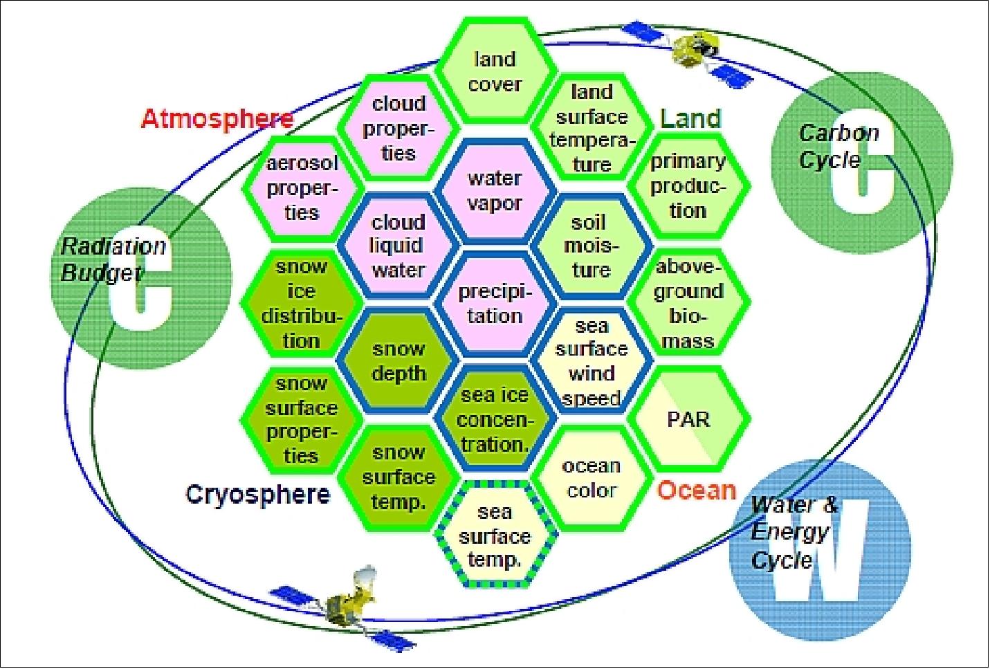
Legend to Figure 2: GCOM-W (blue border) and GCOM-C (green border). SST (Sea Surface Temperature) is observed by both GCOM-W and GCOM-C; hence, its border is a dotted line of blue and green.
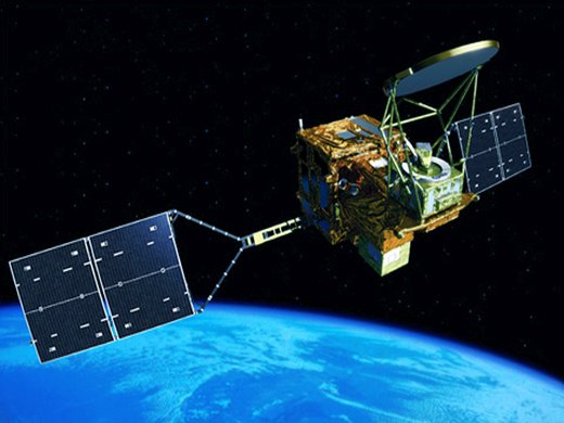
GCOM-W1 (Global Change Observation Mission-Water 1) Mission / Shizuku
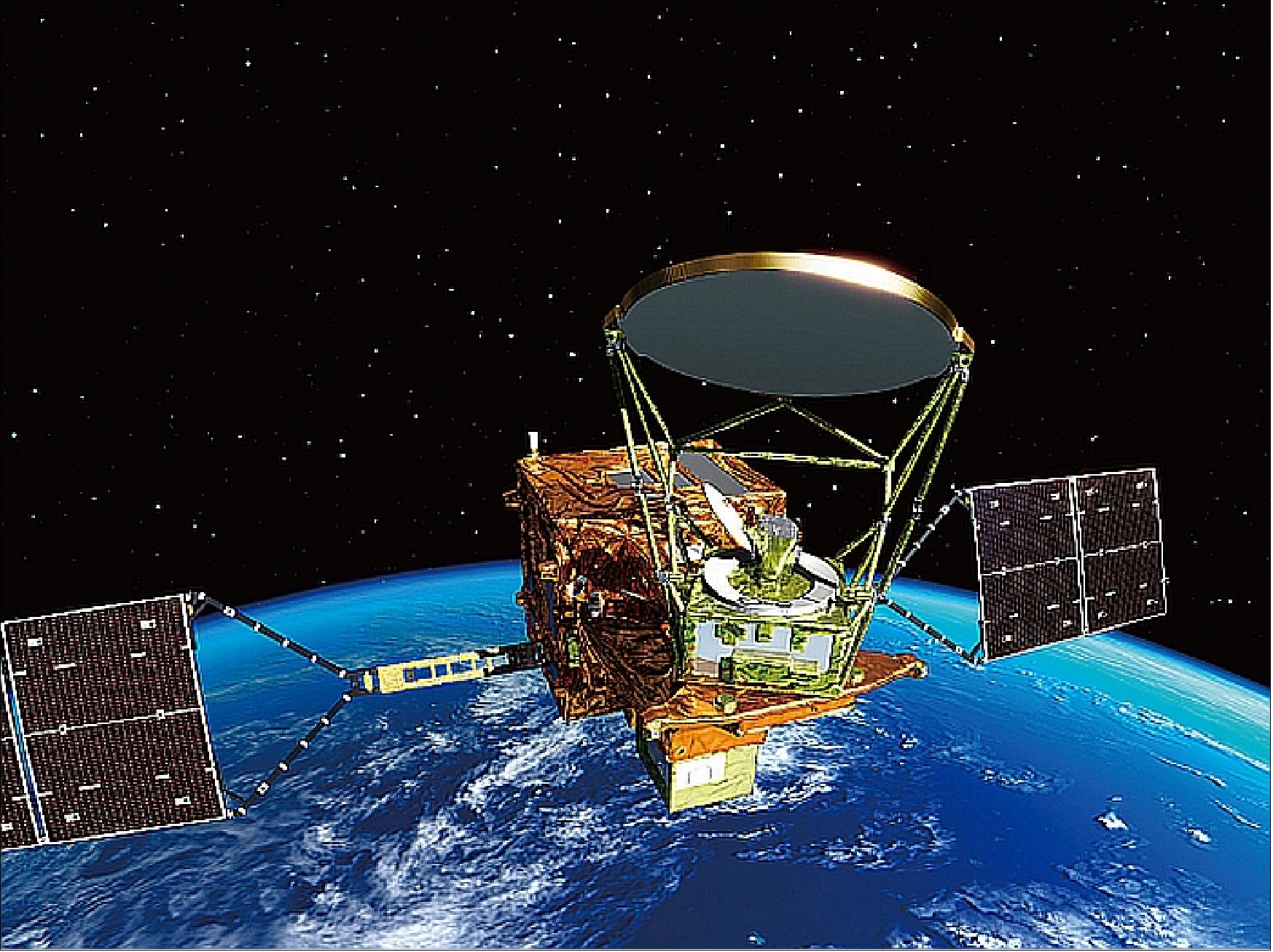
The GCOM-W1 mission of JAXA is dedicated to sea surface monitoring and to contribute to observations related to global water and energy circulation. In September 2011, the GCOM-W1 mission received the nickname Shizuku - meaning a "drop" or a "dew" in Japanese.
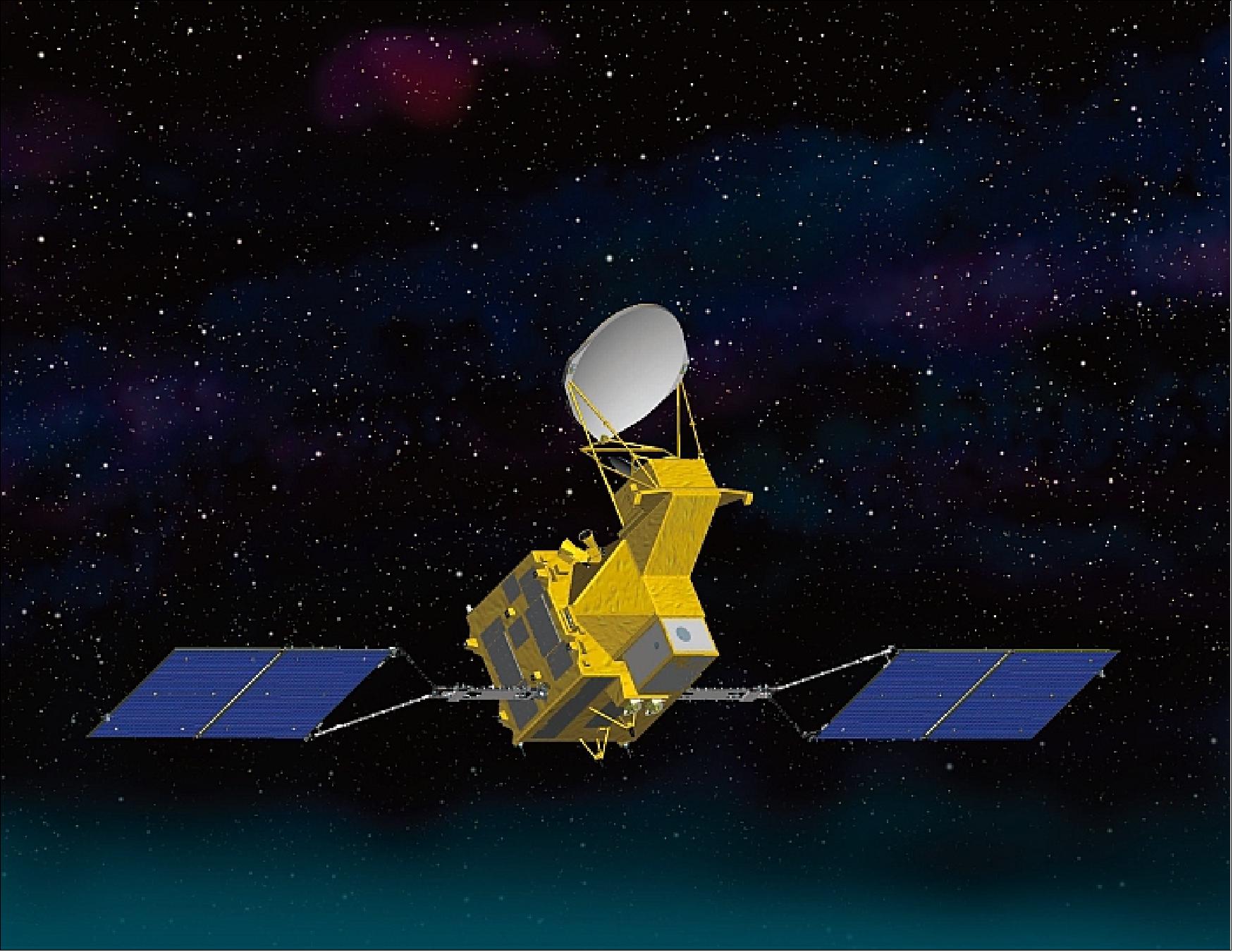
Spacecraft
JAXA has decided to use medium-scale satellites for GCOM series observations. The GCOM-W1 spacecraft is 3-axis stabilized. The attitude of GCOM-W1 is controlled by 4 reaction wheels in response to the signal from IRU (Inertial Reference Unit) calibrated by Star Trackers and GPS receivers.
The EPS (Electrical Power Subsystem) has 2 redundant systems including batteries and solar paddles, and therefore the satellite can survive even if one solar paddle has a failure. Power of 4.05 kW is provided at EOL (End of Life).
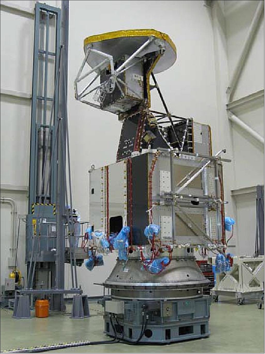
The spacecraft on-orbit dimensions are (deployed configuration): 5.1 m (X) x 17.5 m (Y) x 3.4 m (Z). The spacecraft has a mass of about 1991 kg at launch (dry bus mass of 1324 kg, propellant mass of 151 kg, AMSR2 mass of 405 kg). The design life is 5 years. 18)
The PDR (Preliminary Design Review) of GCOM-W1 took place in March 2008. The spacecraft CDR (Critical Design Review) was completed in December 2009.
GCOM-W1 was integrated in 2010 and has already passed the most of the proto-flight test items in the spring of 2011. The AMSR2 proto-flight model provided desirable characteristics in the ground testing. 19) 20)
RF communications: The S-band is used for TT&C data transmission: TT&C data rates at 29.4 kbit/s (USB), 1 Mbit/s (QPSK,) and 1.6 kbit/s in SSA (S-band Single Access). Command data rates: 4 kbit/s (USB), 125 kbit/s (SSA). The payload data downlink in X-band (8105 MHz) with a data rate of 20 Mbit/s without convolution coding and with the QPSK scheme. Direct real-time downlink of payload data to receiving stations with agreement.
Real-time observation data over Japan are transmitted by X-band to JAXA’s ground stations at Katsuura, or EOC (Earth Observation Center at Hatoyama, Saitama). The received data are distributed immediately after Level-1 data processing.
Launch
The GCOM-W1 spacecraft (nickname: Shizuku - meaning a “drop” or a “dew”) was launched on May 17, 2012 [UTC, the local time in Japan was 1:39 hours on May 18, JST (Japan Standard Time)] on an H-IIA F21 vehicle from TNSC (Tanegashima Space Center), Japan. Launch provider: Mitsubishi Heavy Industries, Ltd. 21) 22)
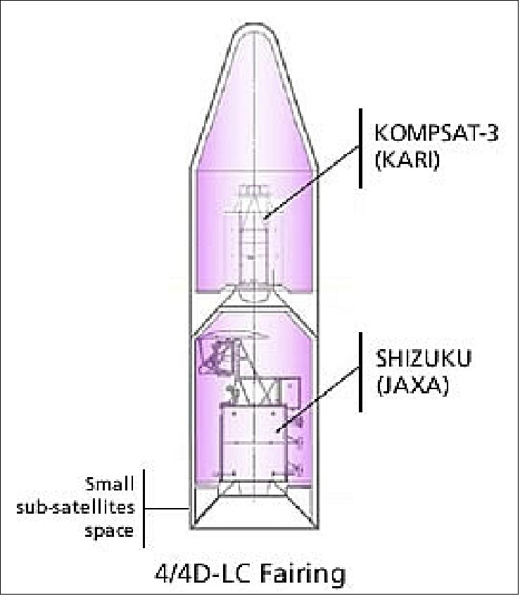
Secondary payloads on this flight were: 24)
• KOMPSAT-3 (Arirang-3) of KARI, Korea with a mass of ~1000 kg. Note: A contract between the launch service provider MHI (Mitsubishi Heavy Industries, Ltd.) and KARI was signed in January 2009. This represents the first satellite launch services order placed to MHI by an overseas customer. 25)
• SDS-4 (Small Demonstration Satellite-4) of JAXA with a mass of ~ 50 kg
• HORUYU-2 of KIT (Kyushu Institute of Technology) with a mass of 7.1 kg.
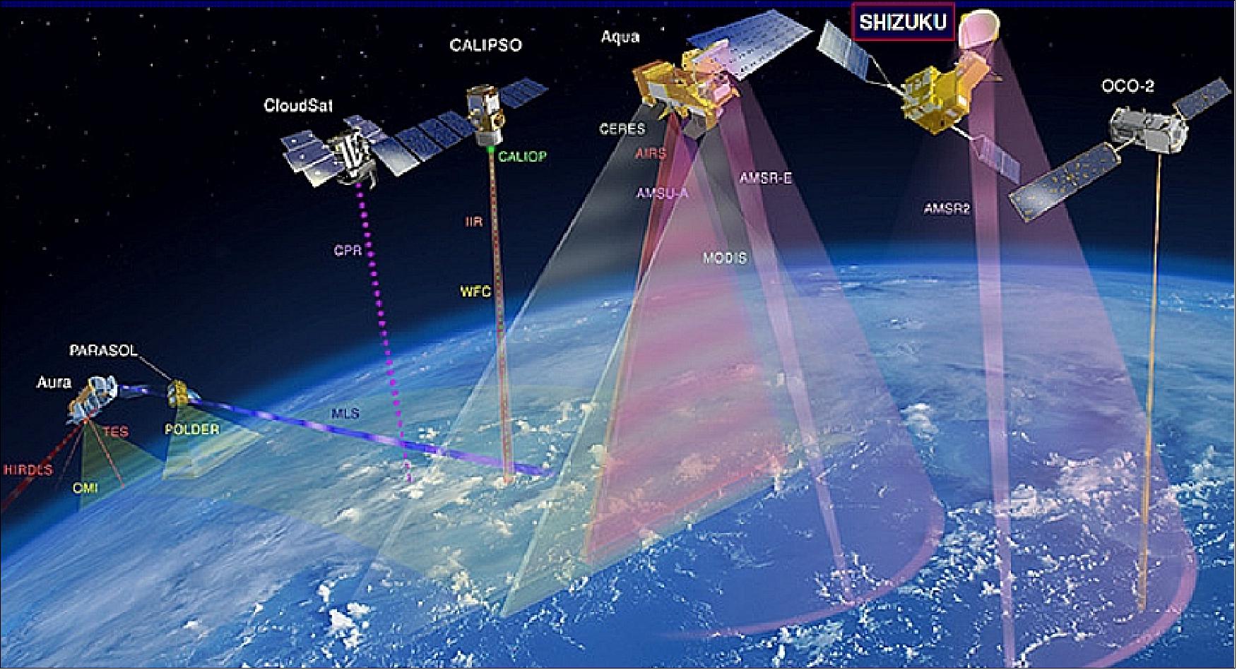
Orbit: Sun-synchronous orbit, altitude = 699.6 km, inclination = 98.2º, LTAN (Local Time on Ascending Node) at 13:30 hours (to continue the AMRS-E observations). Since the orbit is very similar to the one of the A-Train, it will join the A-Train constellation of NASA. The position of GCOM-W1 in the constellation is a few minutes prior to the Aqua spacecraft (Ref. 1). 26) 27)
Mission Status
• February 18, 2020: Australia has naturally faced many droughts and bushfires, but conditions have been unusually severe this time. Sometime around September 2019, the bushfires continuously occurred around the state of New South Wales in southeast Australia. The fires had been spreading on a larger scale, and a number of massive fires had merged into a "Mega Fire" that was out of control. The fires are unlikely to end entirely even at the end of January 2020. 30)
- Bushfires cause not only personal and economic damages, but also environmental degradation for many animals and discharging carbon dioxide to the atmosphere. There are growing concerns about serious damage to habitats for wild animals including koalas, too. This article introduces the results of diversified analysis on the bushfires by using multi-satellite data.
- As seen above, the bushfires have occurred frequently on a widespread basis in Australia since last autumn, especially around the state of New South Wales in the southeast with the condition that the eastern area was extremely dry than average year.
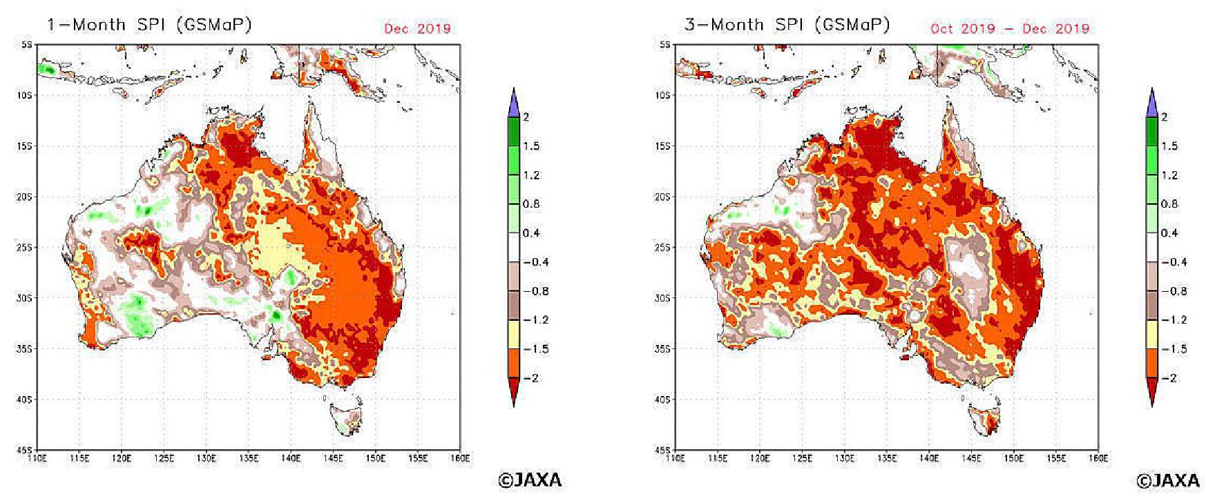
Status of drought: One of the backgrounds of the forest files is the condition of "drought" especially in eastern Australia, which has very little rain compared with normal year. JAXA has generated and provided global precipitation distribution data called "Global Satellite Mapping of Precipitation (GSMaP)" using multiple satellite data, such as the Global Precipitation Measurement(GPM) and Global Change Observation Mission-Water "Shizuku” (GCOM-W). GSMaP data are available since March 2000 and can be utilized in statistical analysis because it has a long-term data set containing satellite precipitation data with less than twenty years. EORC tried to detect drought happened in Australia by calculating Standardized Precipitation Index (SPI) from GSMaP. SPI is the statistical exponent by which we can evaluate drought only using precipitation amount.
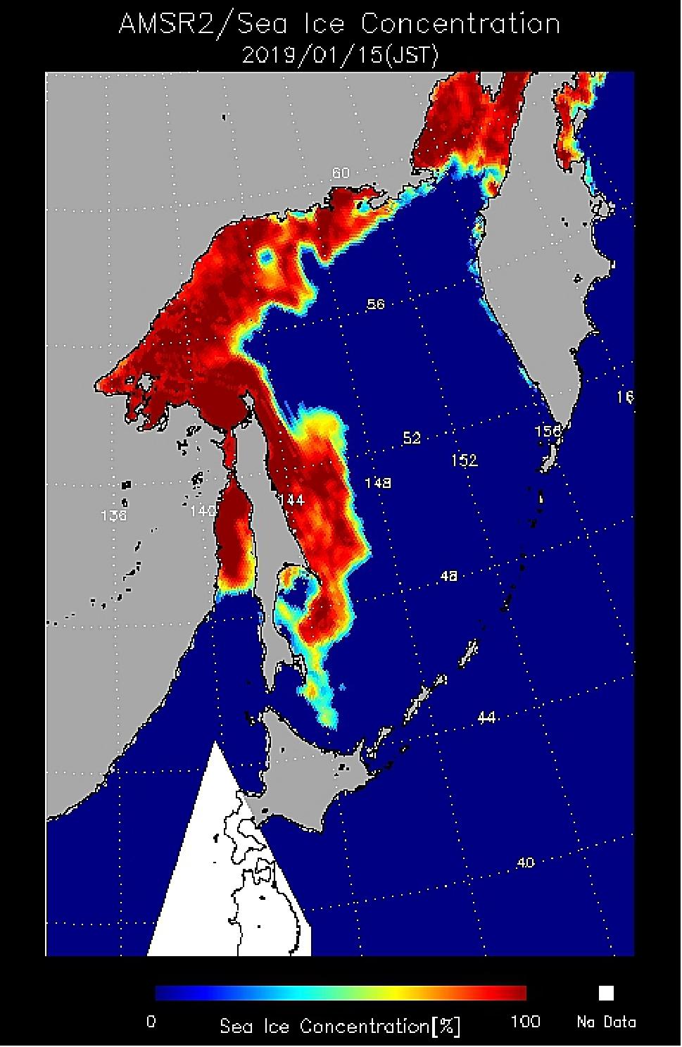
• January 21, 2019: In Hokkaido, drift ice can be seen floating across the Okhotsk Sea, which is located in the northeastern part of Japan. The drift ice season is from January to March, with its peak in February. Drift ice-watching tours start at Hokkaido. 31)
• The GCOM-W satellite and its payload are operating nominally in February 2018. Considering the good health of the satellite and instrument and the status of the onboard consumables, the project plans to continue the GCOM-W mission operations as long as possible to avoid/minimize an observation gap between the AMSR2 (Advanced Microwave Scanning Radiometer-2) and the follow-on sensor. — A major objective of the mission is also to provide continuous observations of the global water cycle succeeding role of JAXA’s AMSR-E (Advanced Microwave Scanning Radiometer - for EOS) on the NASA's Aqua satellite. Note: AMSR-E ended its operational support on 4 Dec. 2015 after more than 9 years of service on Aqua. 33)
- In May 2017, the GCOM-W mission passed its on-orbit design life goal of 5 years.
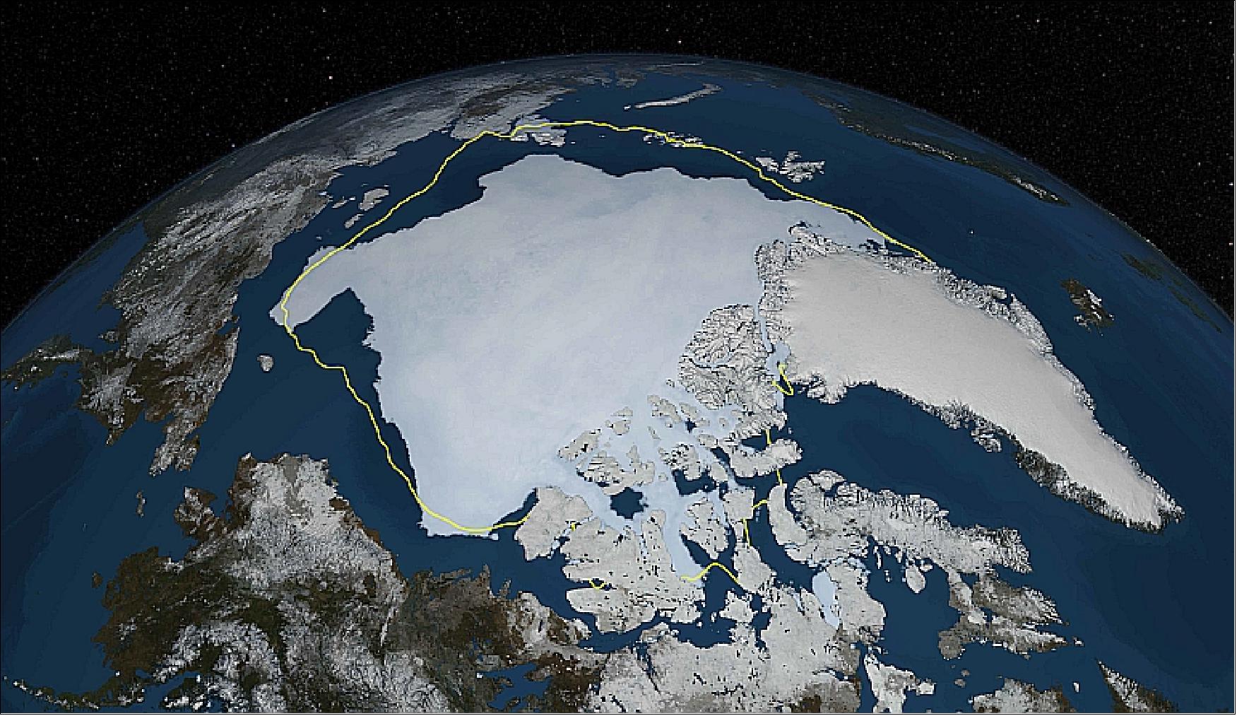
• October 18, 2017: Every year, the process is generally the same: the cap of sea ice on the Arctic Ocean melts and retreats through spring and summer to an annual minimum extent. Then, as the ocean and air cool with autumn, ice cover grows again and the cycle continues. But when we take a look at smaller regions within the Arctic, we get a more detailed picture of what’s been going on. 34)
- The map of Figure 10 shows the extent of Arctic sea ice on September 13, 2017, when the ice reached its minimum extent for the year. Extent is defined as the total area in which the ice concentration is at least 15 percent. The map was compiled from observations by the AMSR-2 (Advanced Microwave Scanning Radiometer 2 instrument on the GCOM -W1 (Global Change Observation Mission 1st-Water)/Shizuku satellite mission operated by JAXA (Japan Aerospace Exploration Agency). The yellow outline in Figure 10 shows the median sea ice extent observed in September from 1981 through 2010.
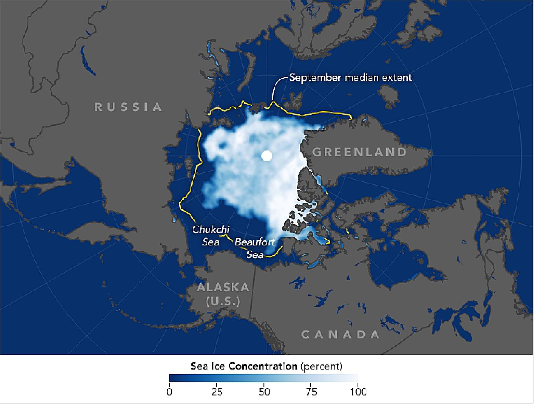
- According to the NSIDC (National Snow and Ice Data Center) in Boulder, CO, the Arctic sea ice cover in 2017 shrank to 4.64 million km2, the eighth-lowest extent in the 39-year satellite record. Charting these annual minimums and maximums has revealed a steep decline in overall Arctic sea ice in the satellite era. But the decline is not the same everywhere across the Arctic Ocean. The Beaufort Sea north of Alaska, for example, is the region where sea ice has been retreating the fastest.
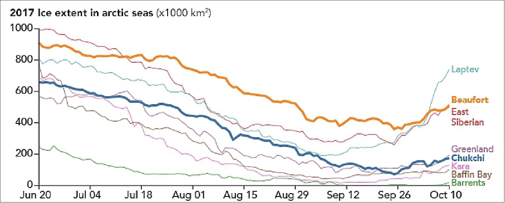
- This year, ice in the Chukchi and Beaufort and seas reached their minimum extents toward the end of September, later than the Arctic as a whole. The graph of Figure 11 shows the ice in these two seas was still declining while other regions had started freezing. The melting persisted the longest in the Beaufort Sea, which finally started to refreeze after reaching a minimum on September 27. Data for the graph come from the NSIDC MASIE (Multi-sensor Analyzed Sea Ice Extent) product, which is based on operational sea ice analyses produced by the U.S. National Ice Center. Note: the MASIE observations included also the SSM/I instrument on the DMSP series. In addition, in situ measurements were used.
- Ice loss is the Beaufort and Chukchi seas was not record-breaking this year, but the extents were much lower than usual. Notice in the map how the ice edge in these seas was farther north than average. According to Walt Meier, a scientist at the NSIDC (National Snow and Ice Data Center), the Chukchi and Beaufort seas entered the melt season with a lot of first-year ice. This ice type is generally thinner than multi-year or perennial ice (which survived the previous melt season); first-year ice tends to melt away more easily.
- Meier also notes that low-pressure weather systems persisted near the North Pole for much of the summer. “Low pressure will keep things cooler overall and generally will lead to a relatively higher ice extent overall,” Meier said. “However, the position of the low this year led to winds blowing from the south and west that help move ice out of these regions. Also, the winds may have helped to bring in warmer ocean waters from the Bering Strait region as well.”
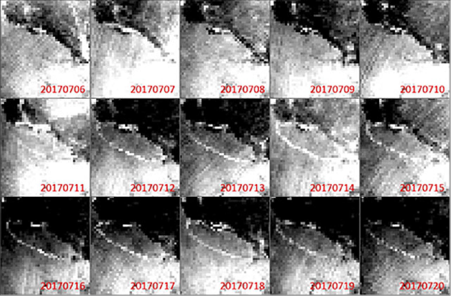
• July 26, 2017: An iceberg about the size of Mie Prefecture of Japan split off from Antarctica’s Larsen C iceberg on July 12, 2017. The AMSR-2 (Advance Microwave Scanning Radiometer-2) on JAXA’s Shizuku satellite captured the calving of the close to 5,800 km2 chunk of ice. The nascent iceberg created by the rift is estimated to weigh over a trillion tons. 35)
- AMSR-2 was instrumental in grasping this major calving event. It can turn to and observe the same area a few times a day regardless of time and weather. Antarctica is currently in its winter, the season of six-month-long darkness. AMSR-2’s high temporal resolution could monitor the progression of the rift despite the absence of light, which the traditional optical sensors cannot.
• In May 2017, the GCOM-W1/Shizuku mission was 5 years on orbit, achieving its design life of 5 years. The project expects that both the satellite and instrument (AMSR2) will continue their operation well beyond this date. 36)
- The AMSR2 standard products have been distributed through the GCOM-W1 Data Providing Service. The system has been in operation since August 2011 to distribute AMSR2 standard products along with AMSR and AMSR-E standard products. Registered users can also use sftp protocol to download data automatically, as well as interactive mode.
- In addition to standard products, registered users can obtain near-realtime data by applying special user form. AMSR2 research product, ASW, has been distributed from the GCOM-W Research Product Data Providing Service (http://suzaku.eorc.jaxa.jp/GCOM_W/) since October 2015.
- For quick look of the products, browse images of all AMSR2 brightness temperatures and geophysical parameters are available at the JAXA Satellite Monitoring for Environmental Studies (JASMES) for Water Cycle (http://kuroshio.eorc.jaxa.jp/JASMES/WC.html).
• February 21, 2017: Global sea ice extent hit record low, according to observations from Shizuku on GCOM (Global Change Observation Mission) on January 14, 2017. It is an all time low in the history of satellite operation that started in 1978, JAXA continues operation of Shizuku and GCOM-C and monitoring arctic sea ice extent, off the coast of Greenland Sea and the rest of the arctic circle. 37)
• The GCOM-W1/Shizuku mission is operational in 2016. 38)
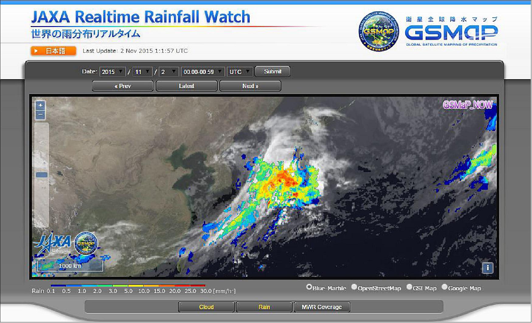
• November 2, 2015: JAXA/EORC (Earth Observation Research Center) has developed GSMaP (Global Satellite Mapping of Precipitation) realtime version (GSMaP_NOW) providing rainfall information of current hour, and released those information through a new webpage “JAXA Realtime Rainfall Watch”. While GSMaP near-real-time version (GSMaP_NRT) is provided with a 4 hour data latency, which consists of 3 hour for data gathering and 1 hour for processing, GSMaP_NOW is provided in quasi-realtime and updated every half hour. For example, hourly GSMaP_NOW image and data during 09:30Z and 10:29Z is available at around 10:30Z through the web site. 39) 40)
- GSMaP_NOW produces rainfall map over the area of geostationary satellite "Himawari", using passive microwave observations that are available within half-hour after observation (GMI, AMSR2 near Japan, and AMSU direct receiving data). Furthermore, half-hour extrapolation of rainfall map toward future direction by using cloud moving vector from the geostationary satellite allows us to estimate "current" rainfall map at every half-hour.
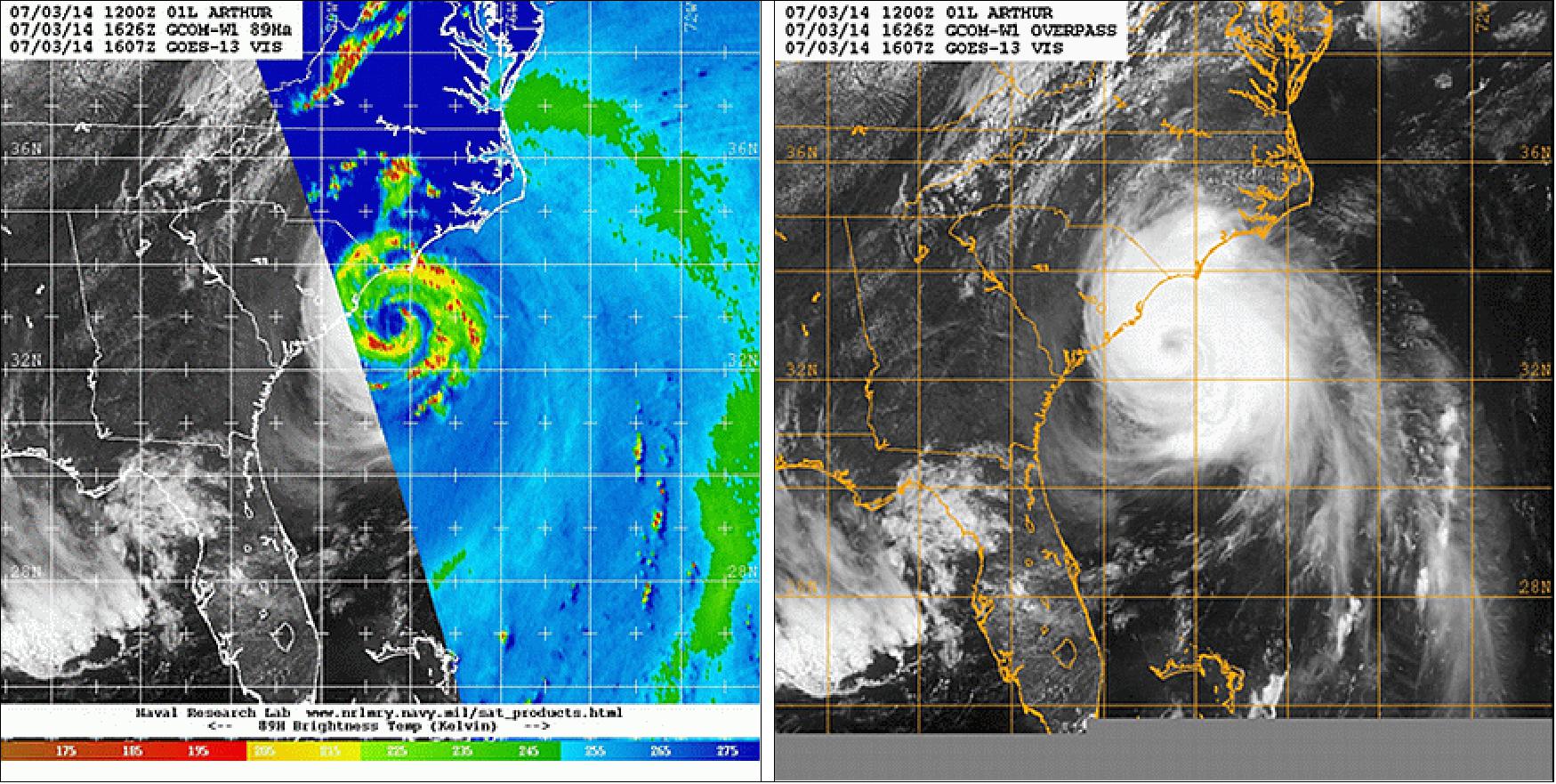
• September 5, 2014: NOAA has begun to routinely utilize observational data acquired by the AMSR2 (Advanced Microwave Scanning Radiometer-2) aboard GCOM-W1/Shizuku to monitor the land, ocean and atmosphere globally and around the U.S. 41)
- NOAA is studying the possibility of utilizing data acquired by the AMSR2 instrument aboard the Shizuku as well as by the DPR (Dual-frequency Precipitation Radar) on the GPM (Global Precipitation Measurement) satellite. Both the AMSR2 and DPR instruments were developed by JAXA, and JAXA and NOAA have been discussing cooperation on the projects. As a first step, AMSR2 data are regularly provided to the U.S. for weather forecast applications. NOAA’s recently signed MOU (Memorandum of Understanding) with NASA on the NASA-JAXA GPM mission will allow NOAA to receive the DPR data. As part of NOAA’s participation with NASA on the GPM Science Team, a few NOAA investigators are testing the feasibility of utilizing the spaceborne radar information from DPR and its predecessor, the PR (Precipitation Radar) flown on the NASA-JAXA TRMM (Tropical Rainfall Measuring Mission) satellite, in regional forecast models to improve the forecasting of tropical systems.
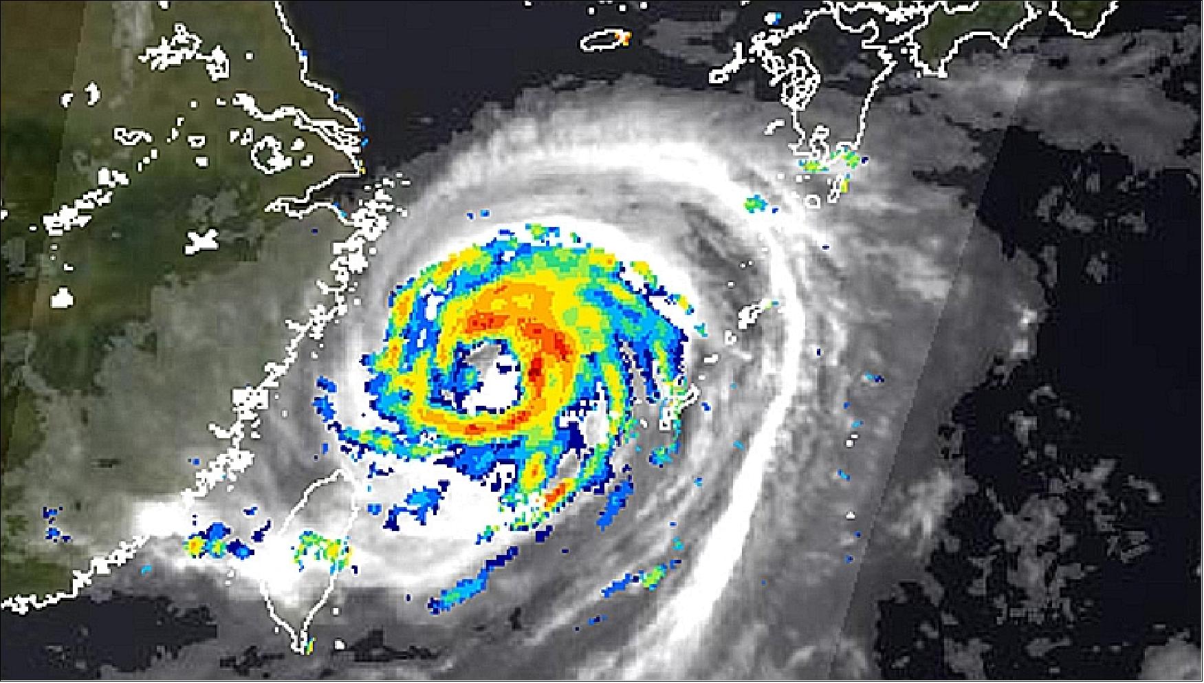
- NOAA’s National Hurricane Center is now routinely utilizing AMSR2 data, which have contributed to improvements in the center location and structure analysis for a number of hurricanes as shown in Figure 16. The cloud image captured through infrared observation (right) cannot clarify the internal structure of a typhoon or hurricane, but the microwave observation (left) clearly shows the dual structure of the eye and surrounding rain bands of Hurricane Arthur off the U.S. East coast through its observation of horizontally polarized brightness temperature (89 GHz-H) being naturally emitted from the Earth's surface and the atmosphere.
• July 2014: GCOM-W1 data is being captured at the KSAT Svalbard ground station and assembled into APID packets. Using the JPSS (NPP) infrastructure, the GCOM raw data APID packets are routed to the NOAA IDPS (Interface Data Processing System) in near-realtime. Once received at the IDPS, the APID packets are reformatted into RDRs (Raw Data Records) and sent to the NDE (NPP Data Exploitation) system for distribution to the Environmental Satellite Data Processing System where further processing to brightness temperatures (Level 1)/SDRs (Sensor Data Records) and geophysical products (Level 2)/EDRs (Environmental Data Records) are performed. The RDRs are processed to SDRs utilizing software provided by JAXA. The EDRs are generated utilizing NOAA's AMSR2 product processing system. - The goal of the product processing system is to provide validated operational L2 products from the AMSR2 instrument that address the GCOM-W1 requirements in the JPSS L1RD supplemental for distribution to operational users. 42)
• July 2014: AMSR2 standard products are distributed through the GCOM-W1 Data Providing Service . Level 1 data has been distributed to public since January 25, 2013, and Level 2 and 3 products since May 18, 2013. The GCOM-W1 Data Providing Service System also distributes AMSR and AMSR-E standard products. Also, registered users can obtain near-realtime data by applying special user form. 43)
• In Feb. 2014, the U.S. NOAA (National Oceanic and Atmospheric Administration) announced that it will utilize observation data acquired by the AMSR2 instrument aboard GCOM-W1, starting in June 2014, to monitor the birth and development of a tropical low pressure system. JAXA and NOAA signed the MOU (Memorandum of Understanding) on GCOM data application in 2011. 44)
• The GCOM-W1 spacecraft and its payload are operating nominally in 2014. 45)
• On Dec. 18, 2013, the JAXA/EORC Tropical Cyclone Database of AMSR2 was released. 46)
• October 17, 2013: The GCOM Project Team of JAXA captured the 2013 Nikkei Global Environmental Technology Awards Prize for Excellence for its development of the Global Change Observation Mission 1st – Water “SHIZUKU” (GCOM-W1). 47)
Legend to Figure 17: The white line shows the 30-year (1981-2010) average minimum extent. The data were provided by JAXA from their Global Change Observation Mission-Water (GCOM-W1) satellite’s Advanced Microwave Scanning Radiometer-2 (AMSR2) instrument.
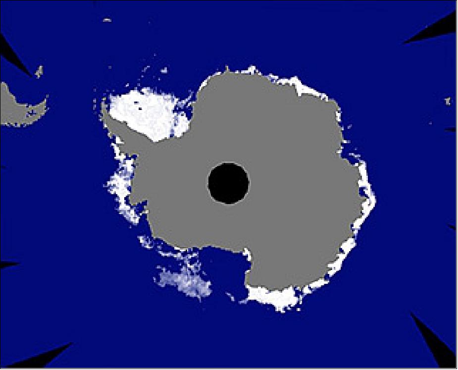
• In late September 2013, the ice surrounding Antarctica reached its annual winter maximum and set a new record. Sea ice extended over 19.47 million km2 of the Southern Ocean. The previous record of 19.44 million km2 was set in September 2012. 49) 50)
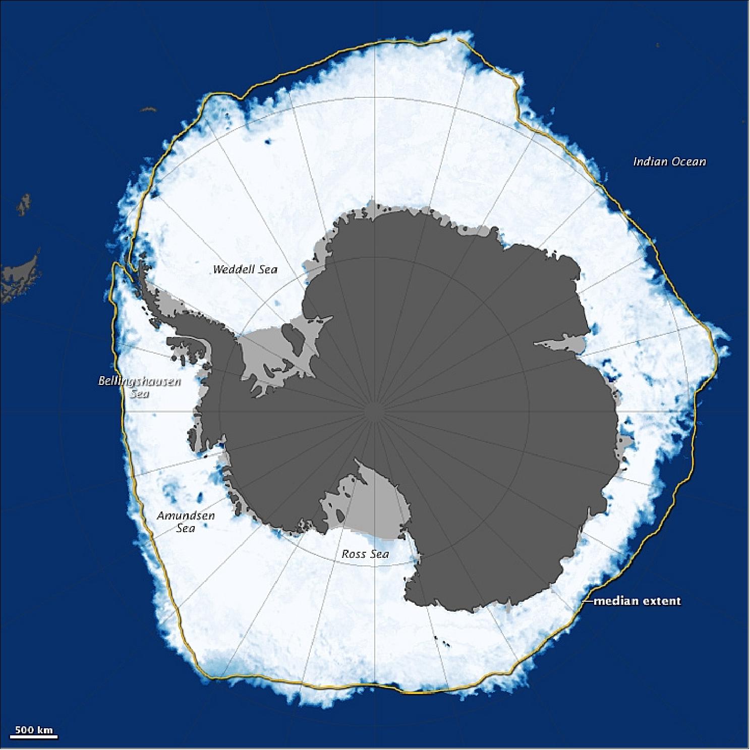
Legend to Figure 18: Antarctica’s sea ice is creeping further out in the ocean! New data from the GCOM-W1 satellite shows that sea ice surrounding the southern continent in late September reached out over 19.47 million km2. The extent — a slight increase over 2012's record of 19.44 million km2 — is the largest recorded instance of Antarctica sea ice since satellite records began, NASA said. While researchers continue to study the forces driving the growth in sea ice extent, it is well understood that multiple factors—including the geography of Antarctica, the region’s winds, as well as air and ocean temperatures—all affect the ice.
• The GCOM-W1/Shizuku spacecraft and its payload are operational in mid-2013. Full operational service (level 2 and level 3 geophysical data products) are available since May 17, 2013. 51)
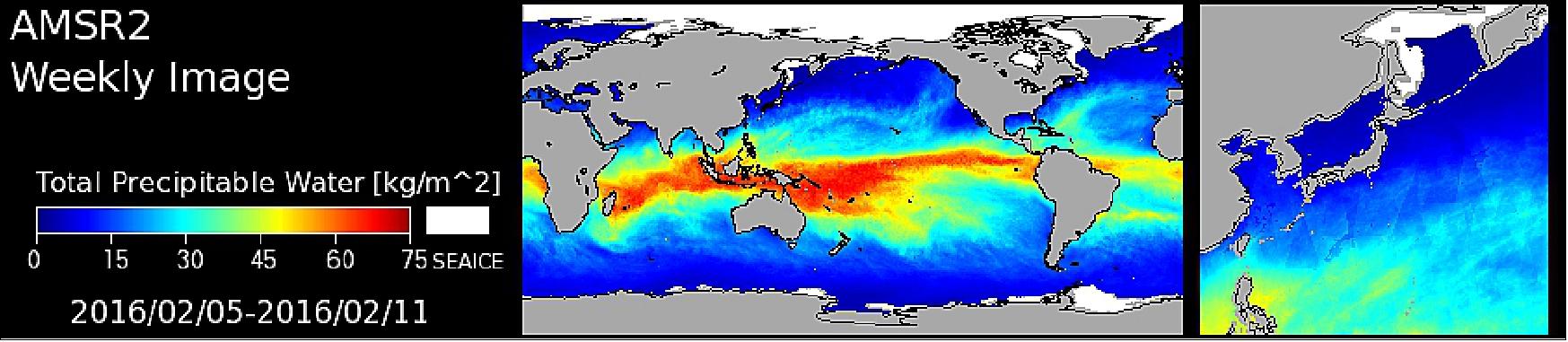
JAXA has started offering eight kinds of products whose physical quantity concerning water on the Earth, including precipitable water and sea surface temperature, is calculated based on the observation data acquired by the AMSR2 (Advanced Microwave Scanning Radiometer 2) aboard the Shizuku (GCOM-W1) after its initial calibration operation was completed. 52)
These products will contribute to capture environmental changes on a global scale such as worrisome decreasing ocean ice areas in the North Pole as well as the El Nino and La Nina Phenomena. The products can also be utilized for various fields including weather and precipitation forecasts for storms and downpours by global meteorological agencies such as the JMA ( Japan Meteorological Agency) and the U.S. NOAA (National Oceanic and Atmospheric Administration).
• In January 2013, JAXA has started offering brightness temperature products from AMSR-2 after its initial calibration operation was completed and the brightness temperature products (level 1B and level 3) with good quality and stability have been available to users at the GCOM-W1 Data Providing Service since late January, 2013. 53)
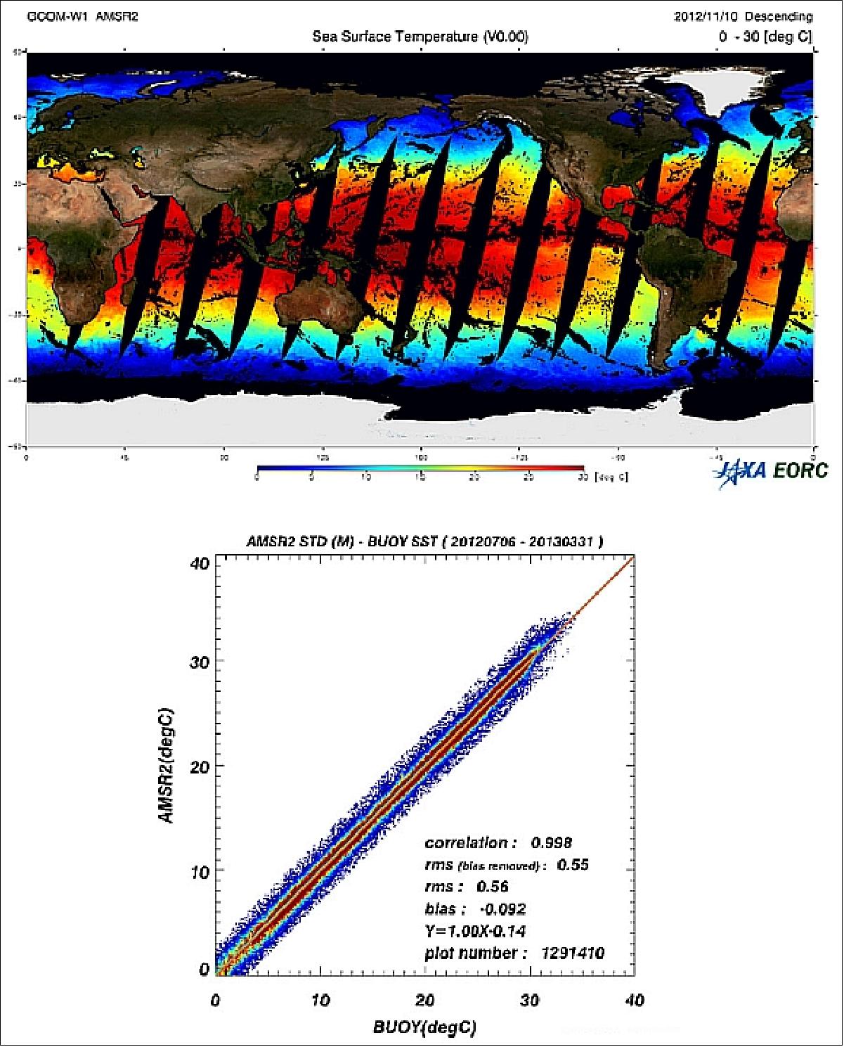
• Nov. 2012: The AMSR2 SST (Sea Surface Temperature) product is validated by comparing with various buoy SST observations reported through the GTS (Global Telecommunication System) operated by WMO (World Meteorological Organization). Each match-up data will include AMSR2 footprints around buoy stations within radius of 30 km and 2 hours. Root mean square error (RMSE) between AMSR2 and Buoy SSTs from August to December 2012 is currently 0.56 °C and correlation coefficient (R) is 0.998 (Figure 19). 54)
• October 2012: JAXA and JAMSTEC (Japan Agency for Maritime-Earth Science and Technology ) are collaborating in the Earth environment field by combining space and oceanic technologies such as merging data acquired by an Earth observation satellite and on-the-spot data obtained through an observation system deployed in the ocean. 55)
The project started to provide data on the Arctic Ocean area acquired by the Shizuku spacecraft to the NiPR (National Institute of Polar Research) for its voyage to observe and investigate the area using JAMSTEC’s Oceanographic Research Vessel “MIRAI”. The provided data is expected to contribute to NiPR’s research and safe navigation. - The project is sending MIRAI data, including sea ice distribution, ocean temperature distribution and sea ice concentrations observed by Shizuku, which can conduct observations regardless of weather conditions, three times a day. Shizuku’s data is being used to find the best sailing routes and for selecting observation areas.
The data on the Arctic Ocean area acquired this time by MIRAI, including the ocean surface temperature, will also be provided to JAXA in order to verify the accuracy of Shizuku’s data as well as to study environment changes such as analyzing recently decreasing Arctic sea ice (Ref. 55).
• On August 10, 2012, JAXA completed the initial functional verification of GCOM-W1 and has moved to the regular observation operation as scheduled. The project will first perform the initial calibration and checkout during which the acquired data will be compared with observation data on the ground to confirming the data accuracy. 56)
- AMSR-2 standard products will be distributed to public for research and educational purposes though web site after calibration/validation phase. The current data distribution schedule (Sept. 2012) is to distribute Level 1 products (brightness temperature) to the public in January 2013, and Level 2 (geophysical parameters) in May 2013. 57) 58)
• July 4, 2012: JAXA released some observation images of Earth acquired by GCOM-W1 (Shizuku). 60)
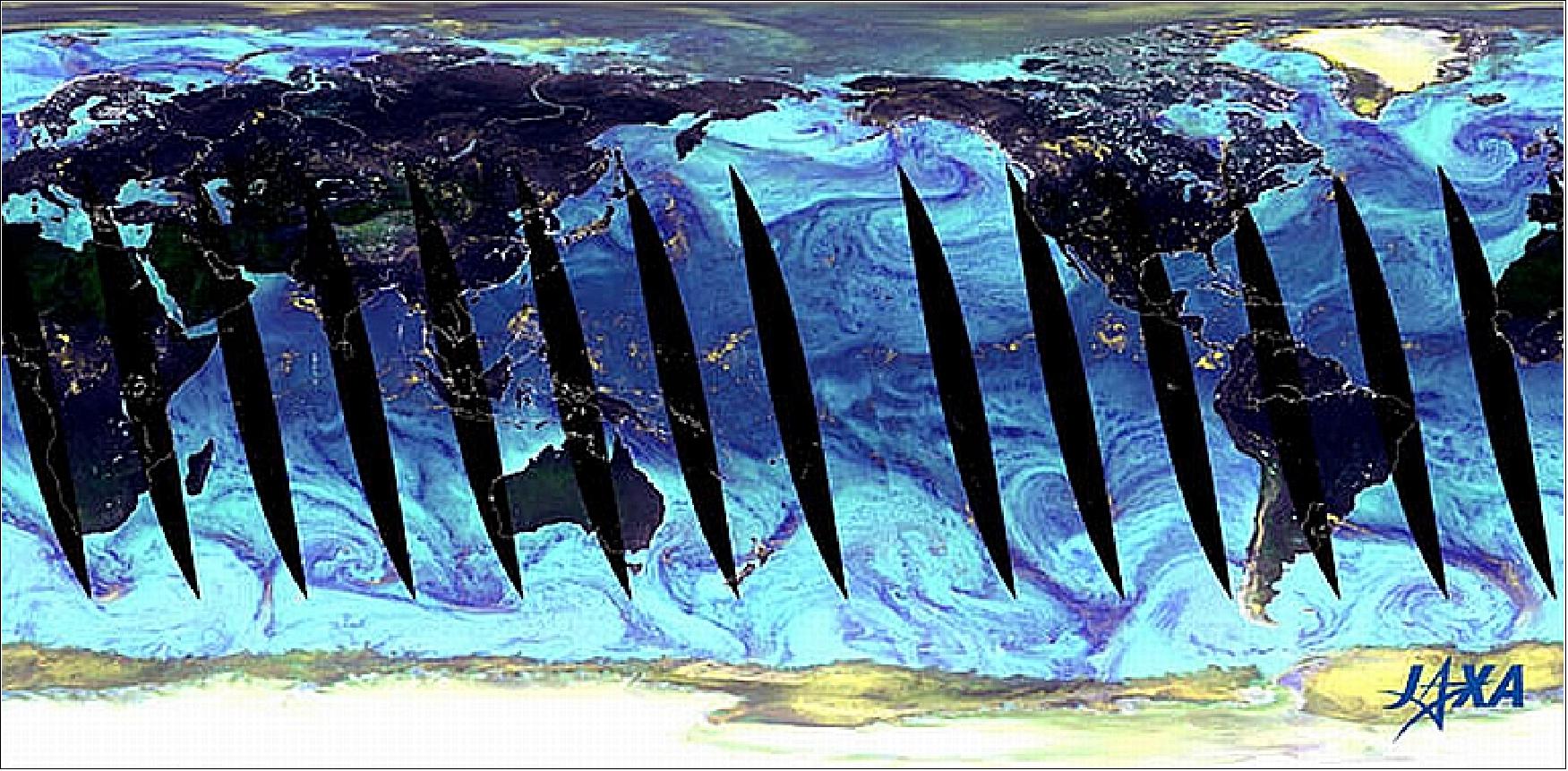
Legend to Figure 22: The one-day image was observed on July 3, 2012 using the brightness temperature (in vertical and horizontal polarization) of the 89.0 GHz channel and the vertical polarization of the 23.8 GHz channel. In this image, whitish-yellow color parts indicate areas with heavy rain or sea ice, light blue color areas are with little water vapor in the atmosphere or thin clouds, the dark blue color sections are areas with more water vapor in the atmosphere or thicker clouds, and the black color parts are areas that were not observed.
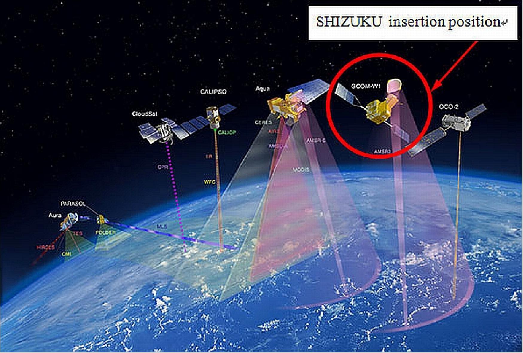
• On June 28, 2012 (UTC), the GCOM-W1 spacecraft was inserted into a planned position on the international A-Train orbit. GCOM-W1 (Shizuku) is flying in front of the Aqua satellite. The satellite will remain in this position until the OCO-2 spacecraft of NASA/JPL joins the constellation sometime in 2014. - JAXA will increase the rotation speed of the AMSR2 aboard the Shizuku from the lower rotation mode (11 rpm) to the regular observation mode of 40 rpm to verify its observation performance. 61)
• JAXA confirmed that the solar array paddle deployment was successfully performed for the Global Change Observation Mission 1st - Water "SHIZUKU" (GCOM-W1) somewhere over Australia via image data. 62)
• After the separation of KOMPSAT-3 spacecraft at 16 minutes into the flight, the GCOM-W1 spacecraft separated from the launch vehicle 23 minutes after launch (Ref. 23).
Sensor Complement
AMSR2 (Advanced Microwave Scanning Radiometer-2)
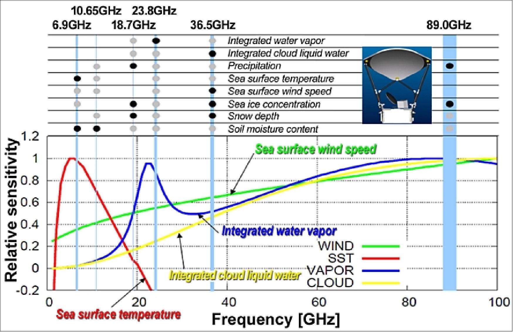
AMSR2 is a follow-on JAXA radiometer of AMSR and AMSR-E heritage (passive instruments) installed on the ADEOS-II (JAXA) and the Aqua (NASA) missions, respectively. The objective is to achieve measurement of: sea surface temperature (SST), soil water content (moisture), sea wind speed, water equivalent of snow cover, precipitation intensity, sea ice distribution, precipitable water, etc. The observables are the microwave emissions from the atmosphere, ocean, sea ice, and land which are being measured at multiple frequencies. 63) 64) 65) 66) 67) 68)
The following improvements of the AMSR2 instrument were implemented based on experience gained in the AMSR-E mission:
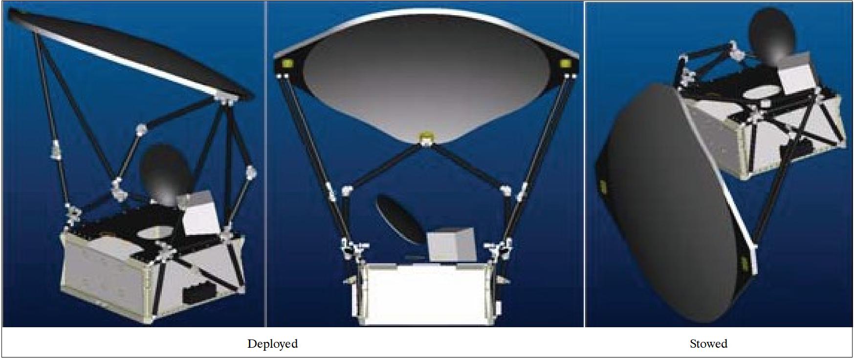
1) Deployable main reflector system with 2.0 m diameter
2) Frequency channel set is identical to that of AMSR-E, except for the additional 7.3 GHz channel for radio frequency interference mitigation
3) Two-point external calibration with the improved HTS. In addition, deep-space maneuver will be considered to check the consistency between the main reflector and CSM (Cold Sky Mirror).
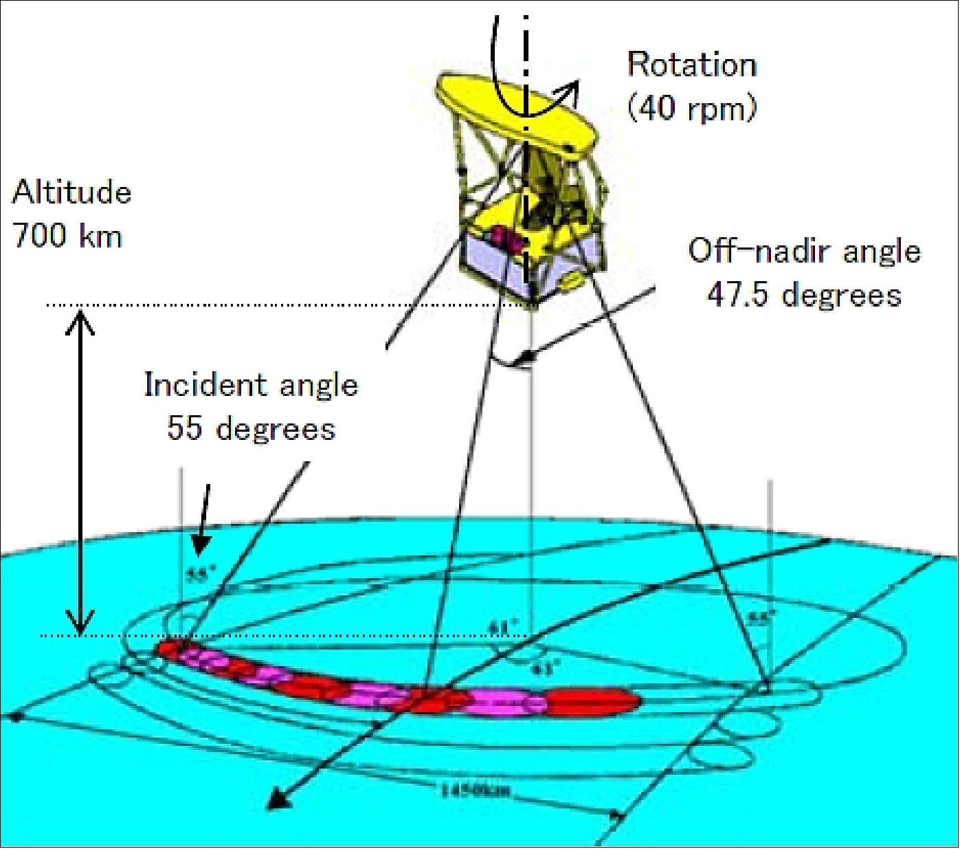
The instrument employs a parabolic offset antenna (antenna aperture of 2 m diameter) providing a conical scan with a swath width of ~ 1450 km (from a 700 km orbit). The incidence angle is 55º nominally. AMSR2 is a total power microwave radiometer with a two point external calibration method:
1) Deep space using a cold sky mirror
2) An on-board hot load.
For the absolute calibration, deep space observations will be done using the main mirror. AMSR2 is able to provide global observations in just 2 days.
The AMRS2 frequency channels are identical to those of AMRS-E except the 7.3 GHz channel which is being used for RFI (Radio Frequency Interference) mitigation in the 6.925 GHz channel. Intensive efforts were made to improve the performance of the HTS (High-Temperature noise Source, a hot load), which has been the greatest challenge in the AMSR-E calibration. A redundant momentum wheel was added to increase the reliability of the instrument.
Center frequency (GHz) | Beam width [Ground resolution (km)] | Bandwidth (MHz) | Sampling interval (km) | Polarization | NEΔT (K) | Data quantization (bit) |
6.925 | 1.8º [35 x 62] | 350 | 10 | V & H | 0.34 | 12 |
7.3 | 1.8º [34 x 58] | 350 | 0.43 | 12 | ||
10.65 | 1.2º [24 x 42] | 100 | < 0.70 | 12 | ||
18.7 | 0.65º [14 x 22] | 200 | < 0.70 | 12 | ||
23.8 | 0.75º [15 x 26] | 400 | < 0.60 | 12 | ||
36.5 | 0.35º [7 x 12] | 1000 | < 0.70 | 12 | ||
89.0 A/B | 0.15º [3 x 5] | 3000 | 5 | < 1.20/1.40 | 12 |
Scan concept | Conical scan at a rotation speed of 40 rpm (1.5 s per scan) |
Swath width | > 1450 km |
Antenna | 2.0 m aperture, offset parabola with a deployable main reflector |
Data quantization | 12 bit |
Incidence angle | 55º nominal |
Polarization | Vertical (V) and horizontal (H) |
Cross polarization | < -20 dB, (< -16 dB for 7.3 GHz) |
Dynamic range | 2.7 K to 340 K |
Sampling interval | 2.6 ms (corresponding to 10 km), 1.3 ms for 89 GHz channel |
Instrument mass | 405 kg |
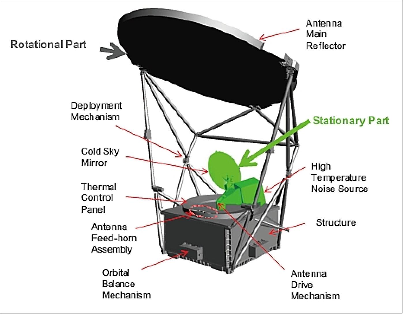
AMSR2 Calibration
AMSR2 has two calibration targets, named HTS (High Temperature noise Source) and CSM (Cold Sky Mirror). The configuration of these targets are shown in Figure 29.
CSM is a 0.6 m diameter offset parabolic reflector, whose manufacturing process is the same as that of the main reflector to ensure consistency between the two reflectors. The antenna patterns of CSM were measured as is the case with main reflector to be verified the performance requirement. In addition to the antenna pattern, VSWR (Voltage Standing Wave Ratio) of the combination of CSM and each feed-horn was measured (Ref. 19).
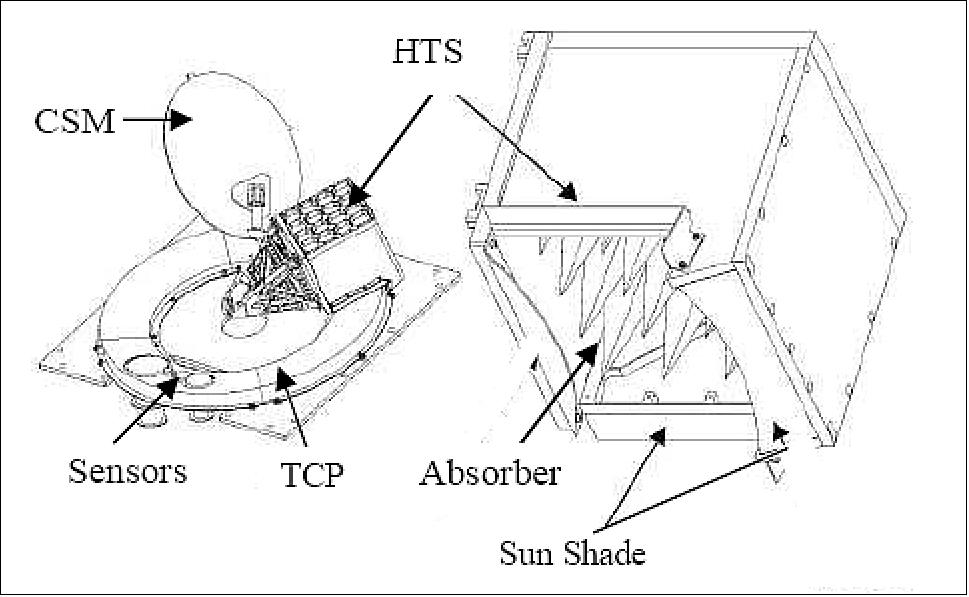
HTS is a microwave absorber shrouded in a thermally-controlled box and panel. HTS/AMSR2 thermal design: The accuracy and the reliability of AMSR2 has been improved compared with the designs of AMSR and AMSR-E. There were major problems in HTS thermal design of AMSR and AMSR-E,and they caused large temperature gradient on the absorber surface of HTS. For the thermal design of HTS/AMSR2, the following two major items were requested to improve: (Ref. 64)
1) Uniformity of the absorber surface (2.5ºCp-p)
2) Thermal measurement accuracy (0.4ºC (3σ)).
Uniformity of the absorber surface of HTS/AMSR2.
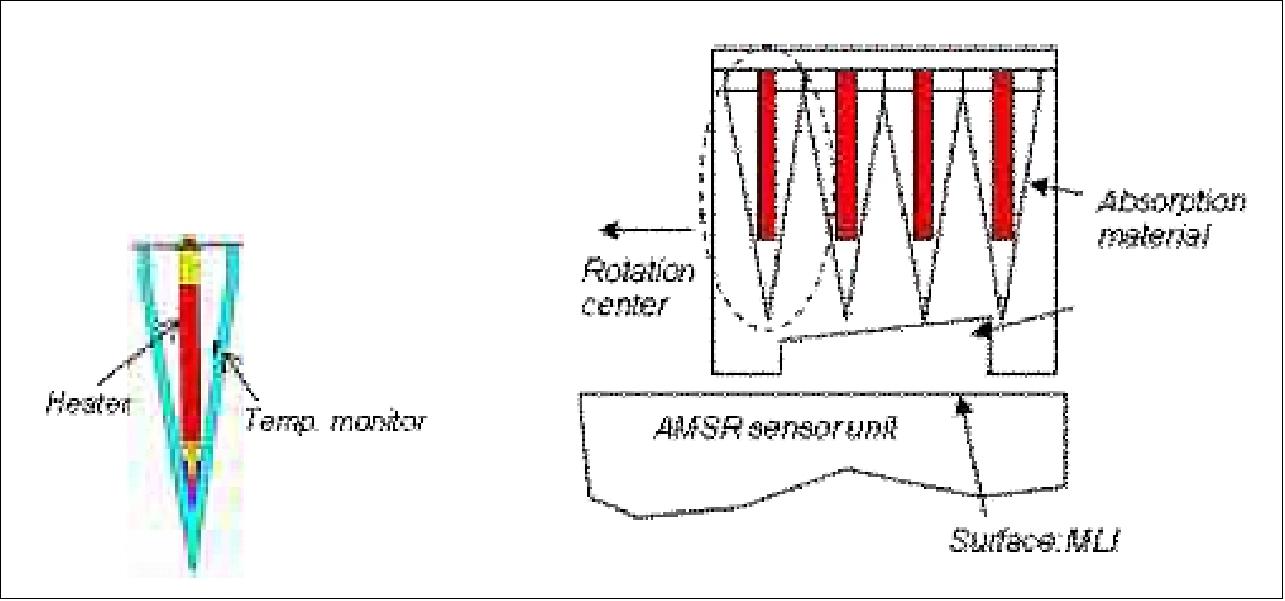
To improve the temperature uniformity, thermal design of HTS/AMSR2 has been improved. The thermal design of HTS/AMSR, AMSR-E, shown in Figure , has the following features:
- Controlling the absorber temperature using heater rods inside the absorber corns
- The surface at the facing side of the absorber covered with MLI whose temperature was not controlled.
- The thermal connection between the absorber surface and outside(space, sun etc.) was large because there were big chinks between HTS and the MLI of the facing side. This design caused the large temperature gradient on the absorber surface.
The improved thermal designed was analyzed using on-orbit thermal analysis and two thermal vacuum tests. As a result of the on-orbit thermal analysis with the AMSR2 model, which adopted these improvements, the temperature uniformity of the absorber is satisfying the request.
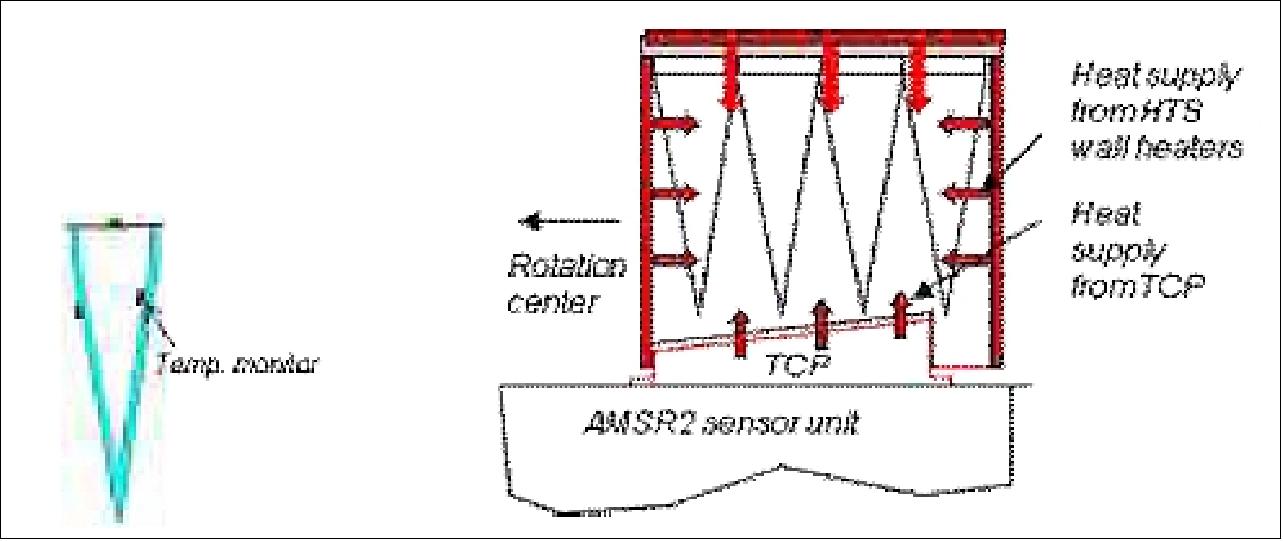
To improve the temperature uniformity of its surface, The thermal design around HTS/AMSR2 had been improved in the following items (shown in Figure 31):
- Changing thermal control methodology; covering all aspects of the absorbers with panels whose temperatures are uniformly controlled. (instead of the Heater rod in the AMSR-E/HTS)
- Installing the TCP (Thermal Control Panel) to control the temperature of the facing side of absorber surface
- Installing “Sun Shade” to minimize the sunlight heat input which comes into HTS through the chinks between HTS and TCP.
Characterization and Calibration of Early Orbit Data
By the extensive effort in improving HTS in terms of thermal control mechanism, in-orbit performance of HTS was significantly improved. Therefore, the project applies the simple two-point calibration method for deriving AMSR2 Tbs in the current processing system, with corrections such as for detector non-linearity and antenna beam characteristics (e.g., spillover factor and cross-polarization ratio), based on the pre-launch laboratory measurements and analyses. Also, the measured antenna patterns were used in deriving coefficients to produce Level-1R product. Although the satellite system was designed to enable deep space calibration maneuver during the initial checkout phase, it was cancelled because of the potential risk of strong RFI which could damage the AMSR2 receivers (Ref. 71).
Intercalibration with Other Microwave Radiometers
Currently (2013), the project is testing several intercalibration methods for version 1.1 AMSR2 Tbs. The first one is to intercalibrate multiple polar orbiting microwave radiometers by utilizing the TRMM (Tropical Rainfall Measuring Mission) TMI (Microwave Imager) as a transfer radiometer. Since TMI can cover various observing local time by TRMM’s precession orbit, one obtains simultaneous observations by TMI and each polar orbiting radiometer and then indirectly compare among polar orbiting radiometers via TMI.
The same concept has been studied and tested by GPM X-CAL team. Because of different sensor characteristics such as in the observing center frequency and Earth incidence angle, these differences must be compensated before comparison. To do this, RTMs (Radiative Transfer Models) are being used and global analysis data produced by meteorological agencies. The project is currently using RTTOV 10.2 distributed by the Satellite Application Facility for Numerical Weather Prediction as RTM 6). In simulating Tbs, we are usingsurface emissivity model/atlas built-in RTTOV10.2: FASTEM 5 for ocean and TELSEM for land surface emissivity. We are using ERA-Interim analysis produced by the European Centre for Medium-Range Weather Forecasts and the Global Daily Sea Surface Temperatures produced by the Japan Meteorological Agency. The analysis procedure is as follows for the case of AMSR2 and TMI intercalibration.
- Create spatio-temporal match-up Tb dataset between AMSR2 and TMI observations.
- Compute differences between observed and calculated Tbs (O-C) for both AMSR2 and TMI, over rainforest and cloud-free/calm ocean areas. Global analysis data and RTM are used to derive calculated Tbs.
- Further create “double difference” to cancel out the differences in frequency and incidence angle: AMSR2 (O-C) – TMI (O-C).
Data Products
The following parameters are part of the GCOM-W1 standard products: 70)
• Brightness temperature
• Total vapor power
• Total cloud liquid water
• Precipitation
• SST (Sea Surface Temperature)
• Sea surface wind speed
• Sea ice concentration
• Snow amount
• Soil moisture
Products | Observation areas | Resolution | Accuracy | Range | ||
Release | Standard | Goal | ||||
Brightness temperature (Tb) | Global | 5-50 km | ±1.5 K | ±1.5 K | ±1.0 K (systematic) | 2.7 - 340 K |
Integrated water vapor (TPW) | Global, over ocean | 15 km | ±3.5 kg/m2 | ±3.5 kg/m2 | ±2.0 kg/m2 | 0 - 70 kg/m2 |
Integrated cloud liquid water (CLW) | Global, over ocean | 15 km | ±0.10 kg/m2 | ±0.05 kg/m2 | ±0.02 kg/m2 | 0 - 1.0 kg/m2 |
Precipitation (PRC) | Global, except cold latitude | 15 km | Ocean ±50% | Ocean ±50% | Ocean ±20% | 0 - 20 mm/h |
SST (Sea surface temperature) | Global, over ocean | 50 km | ±0.5ºC | ±0.5ºC | ±0.2ºC | -2 - 35ºC |
Sea surface wind speed (SSW) | Global, over ocean | 15 km | ±1.5 m/s | ±1.0 m/s | ±1.0 m/s | 0 - 30 m/s |
Sea ice concentration (SIC) | Polar region, over ocean | 15 km | ±10% | ±10% | ±5% | 0 - 100% |
Snow depth (SND) | Land | 30 km | ±20 cm | ±20 cm | ±10 cm | 0 - 100 cm |
Soil moisture (SMD) | Land | 50 km | ±10% | ±10% | ±5% | 0 - 40% |
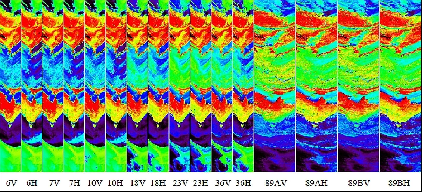
Product level definition: Table 2 shows a definition of AMSR2 processing levels. Tb products are available in three processing levels: Level-1B, -1R, and -3. The Level-1B product contains Tb values in swath format with native spatial resolution of each frequency channel. On the other hand, the Level-1R product provides resolution-matched Tbs by some sort of beam pattern matching procedure with the Backus-Gilbert method . Because of the significant differences in the spatial resolution, it is not straightforward to combine Tbs at different frequency channels. This Level-1R product aims to ease this difficulty for data users. Four resolution sets (6, 10, 23, 36 GHz) and raw swaths of 89 GHz A/B scan are included in a Level-1R granule. For example, in the 10.65 GHz resolution set, Tbs at 10.65, 18.7, 23.8, 36.5, and 89.0 GHz channels are stored, by lowering the spatial resolutions of the channels at 18.7 GHz and higher. Spatio-temporally averaged Tbs are available in the Level-3 product at 0.1/0.25 degrees and 10/25 km resolutions in the equidistant cylindrical and polar stereo projection methods, respectively. 71)
Processing level | Contents |
Level-1A | - Swath data with geolocation information |
Level-1B | - Swath data with geolocation information |
Level-1R | - Swath data with geolocation information |
Level-2 | - Swath data with geolocation information |
Level-3 | - Grid data with 0.1/0.25 degrees (10/25 km) resolution |
Assessment of the C-band RFI (Radio Frequency Interference)
Figure 32 shows the spatial distribution of the Tb difference between 6.925 and 7.3 GHz vertical polarization channels. Since the frequency difference of these two bands are small, the Tbs emitted from natural targets should be similar. Therefore, large differences may indicate potential RFI signals, although these differences in some areas such as over ice sheet and intense precipitation areas may be the real natural signal. In Figure 32, the red color (blue color) indicates the area where Tbs at 6.925 GHz (7.3 GHz) are potentially contaminated by RFI. A significant amount of RFI signatures over the U.S., Japan, and some parts of Europe to India in the 6.925 GHz vertical polarization channel is similar to those of AMSR-E. The RFI signatures at the 7.3 GHz channels seem to be more widespread. Over land, they are evident over Southeast Asia, Eastern Europe, Russia, and so forth. Also, the frequency of occurrences of the 7.3 GHz RFI is higher over the ocean. However, the most important fact is that the spatial distributions of the RFI signatures at these two bands are quite different. Also, there are still many areas with small Tb difference between the two bands, indicating the areas free from RFI (Ref. 71).
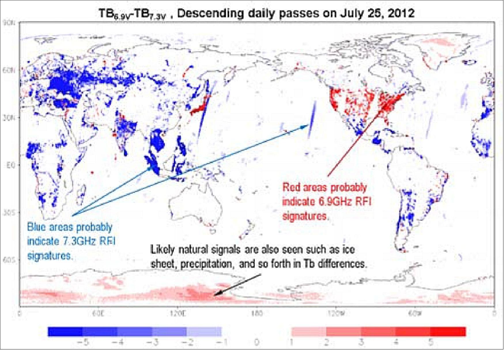
Figure 33 shows statistics of Tb difference between 6.925 and 7.3 GHz vertical polarization channels from July 2012 to January 2013. From the average panel (upper left), the same characteristics can be confirmed as in Figure 32. Typical RFI signatures indicate periodical fluctuations, some from actual time variations and some from observing the azimuth angle dependence. Therefore, the standard deviation panel (lower felt) also indicates potential RFI signatures.
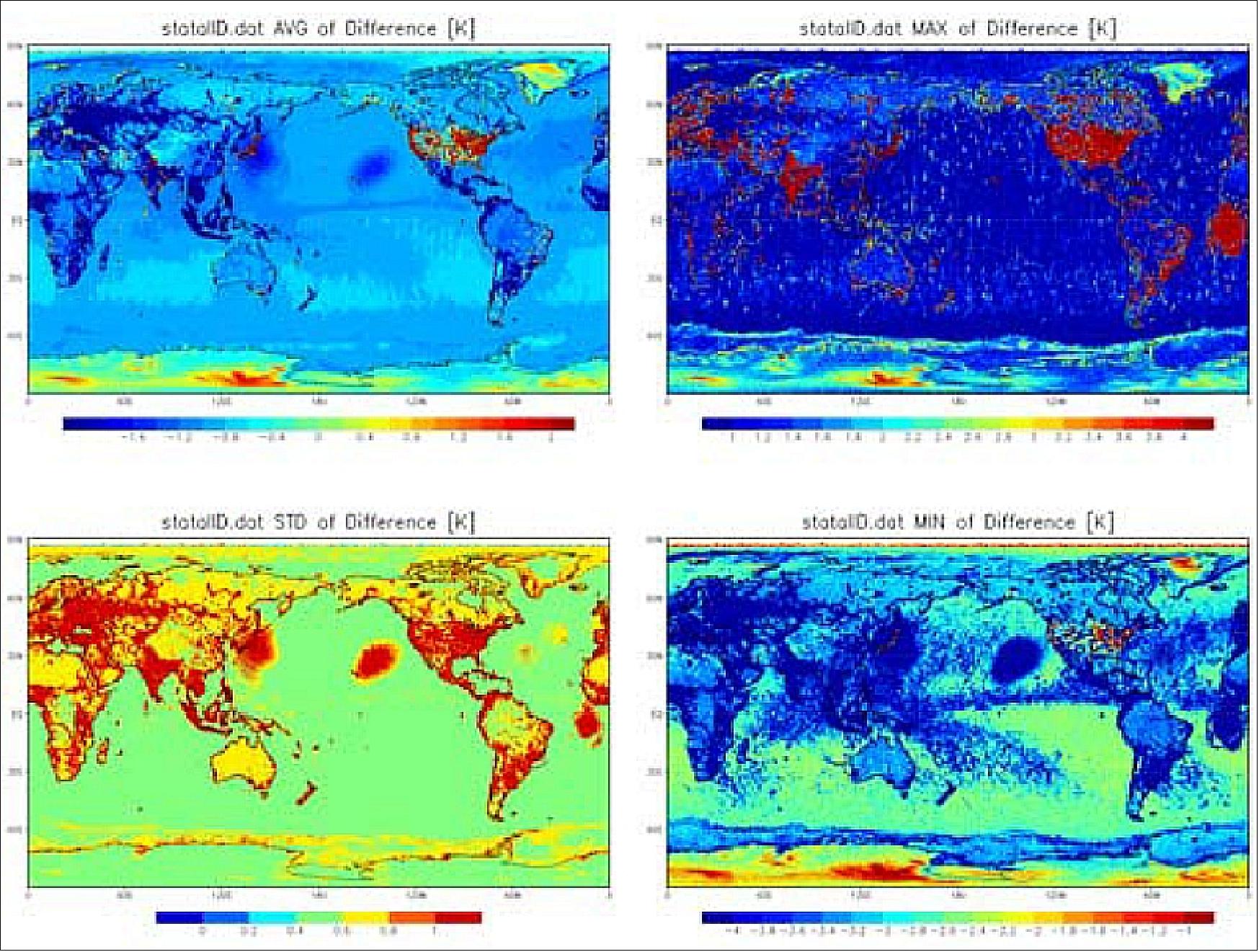
The maximum (upper-right) and minimum (lower-right) panels show potential RFIs in 6.925 and 7.3 GHz channels, respectively. In addition to RFI over land, clear signatures can be found over ocean, particularly around Japan and Hawaii in the 7.3 GHz channel, and around Ascension island in the 6.925 GHz channel. As shown in the minimum panel over the tropical to mid-latitude areas, Tbs at 7.3 GHz channel are much more sensitive to precipitation signals than at 6.925 GHz. On the other hand, the Tbs at the 6.925 GHz channel are significantly higher than those at the 7.3 GHz channel over the Antarctic and Greenland ice sheets, indicating volume scattering. Probably for similar reasons, the Tbs at 6.925 GHz are slightly higher over the desert, Tibetan Plateau, and high-latitude land regions. Those natural signals should be distinguished from the RFI signals. Currently, the project is testing simple RFI identification methods by using the Tb difference between the 6.925 and the 7.3 GHz channels. The method seems to work well over the United States, where the RFI at the 6.925 GHz channel is dominant. However, it may not work over the areas with RFIs at both frequency channels, such as Eastern Europe and India. To construct a robust method of RFI identification, it would be necessary to use other channels in combination with the Tb difference between the 6.925 and 7.3 GHz channels. The project is working on the revised method to flag the RFI contaminated footprints (Ref. 71).
Ground Segment
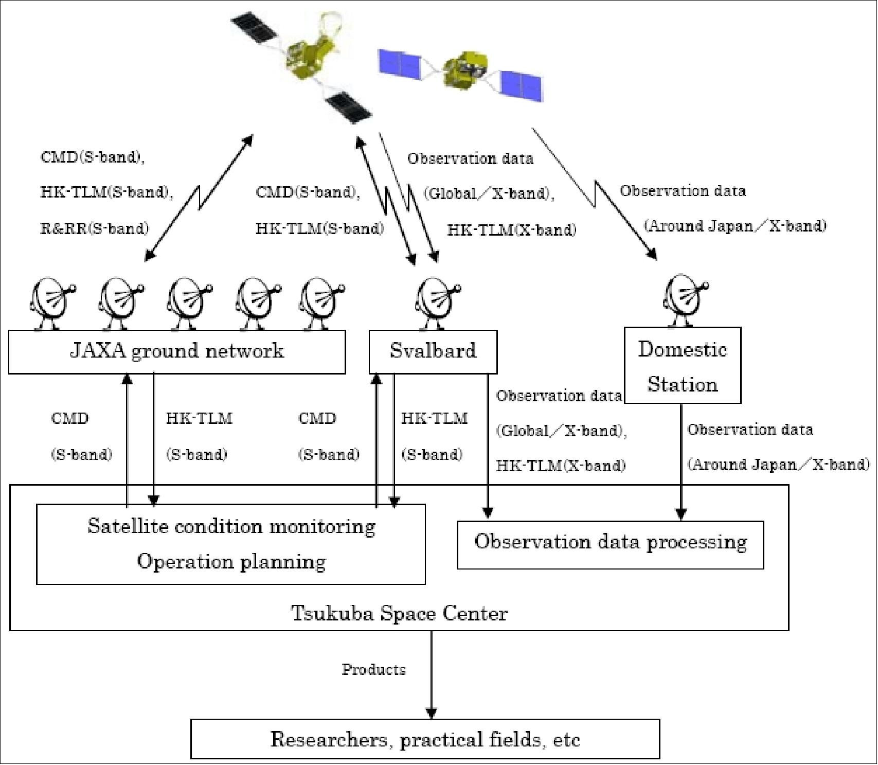
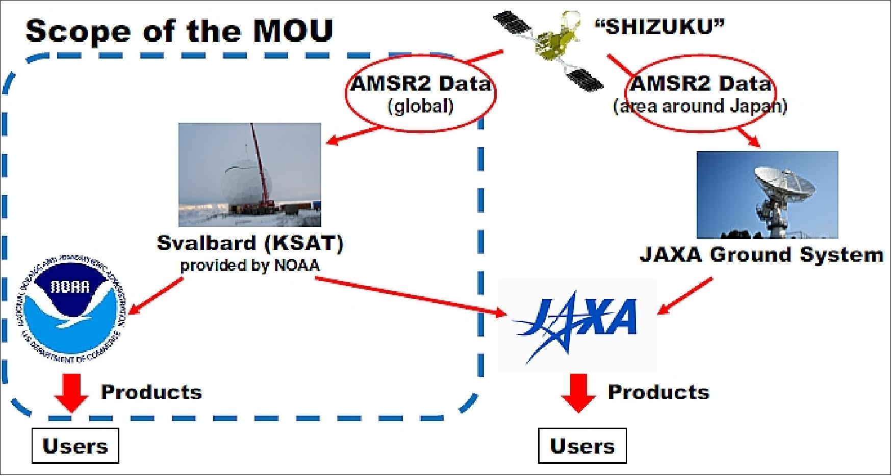
There will be two categories of observation data from the GCOM payload instruments: a) the global observation data set, which will be downlinked to the Svalbard station (Spitzbergen, Norway) on every orbit; b) the regional observation data around Japan (a subset), which will be downlinked to the JAXA domestic station on every pass of station visibility.
• The global observation data will be sent from Svalbard to TKSC (Tsukuba Space Center). They will be archived and processed at TKSC and be delivered to researchers and practical fields users.
• The regional observation data around Japan will be sent from the JAXA domestic station to TKSC. They also will be archived and processed at TKSC and be delivered to researchers and practical fields users.
JAXA will provide JMA (Japan Meteorological Agency) and JAFIC (Japan Fisheries Information Service Center) with the observation data of AMSR2 and SGLI, respectively. JMA and JAFIC will use them for weather forecast and sea condition information, respectively.
The TT&C (Telemetry Tracking & Command) data will be downlinked to Svalbard via X-band, and to the JAXA ground network via S-band, and be sent to TKSC. TKSC is in charge of spacecraft monitoring and control including operations planning.

In an international partnership agreement, JAXA will provide GCOM-W and GCOM-C observation data to NOAA for the continuity of NOAA user needs. 72) 73) 74)
• The AMSR2 may serve as a potential substitute for JPSS (Joint Polar Satellite System), the former NPOESS MIS (Microwave Imager Sounder).
• SGLI (Second Generation Global Imager) to provide ocean color capability not accomplished by NPP, plus augment other VIIRS capabilities.
GCOM-W and -C cooperation directly contributes to the Disaster, Water, Weather and Climate SBA (Societal Benefit Areas) by providing critical meteorological, climate and environmental observation data. The cooperation also will contribute indirectly to the other SBAs of Health, Energy, Ecosystem, Agriculture and Biodiversity.
References
1) Keizo Nakagawa, “Global Change Observation Mission (GCOM),” Proceedings of ISPRS (International Society for Photogrammetry and Remote Sensing) Technical Commission VIII Symposium, Kyoto, Japan, Aug. 9-12, 2010, URL: http://www.isprs.org/proceedings/XXXVIII/part8
/headline/JAXA_Special_Session%20-%201/JTS12_20100306153736.pdf
2) T. Igarashi, “Global Change Observation Mission-Climate (GCOM-C),” Proceedings of ISPRS (International Society for Photogrammetry and Remote Sensing) Technical Commission VIII Symposium, Kyoto, Japan, Aug. 9-12, 2010, URL: [web source no longer available]
3) T. Sasaki , K. Nakagawa, “GCOM Mission Overview,” Proceedings of the 26th ISTS (International Symposium on Space Technology and Science) , Hamamatsu City, Japan, June 1-8, 2008
4) Information provided by Keizo Nakagawa of JAXA, Tokyo, Japan
5) K. Imaoka, “Status of the GCOM-W mission and AMSR follow on instrument,” AMSR-E Joint science team meeting ,University of Hawaii at Manoa, August 13, 2005 URL: [web source no longer available]
6) H. Shimoda, “Global change observation mission,” URL: http://www.cosis.net/abstracts
/COSPAR2006/00204/COSPAR2006-A-00204.pdf?PHPSESSID=7d14646d7a0631d1dc351ad1f55d038b
7) http://www.jaxa.jp/projects/sat/gcom/index_e.html
8) H. Shimoda, “Global Change Observation Missions,” Proceedings of the 32nd ISRSE (International Symposium on Remote Sensing of Environment), San José, Costa Rica, June 25-29, 2007
9) H. Shimoda, “Global Change Observation Missions,” Proceedings of IGARSS 2007 (International Geoscience and Remote Sensing Symposium), Barcelona, Spain, July 23-27, 2007
10) http://www.jaxa.jp/pr/brochure/pdf/04/sat25.pdf
11) Haruhisa Shimoda, “Overview of GCOM,” Proceedings of IGARSS (IEEE International Geoscience and Remote Sensing Symposium) 2010, Honolulu, HI, USA, July 25-30, 2010
12) Haruhisa Shimoda, “Overview of GCOM,” Proceedings of IGARSS (IEEE International Geoscience and Remote Sensing Symposium), Melbourne, Australia, July 21-26, 2013
13) Misako Kachi, Keiji Imaoka, Hideyuki Fujii, Daisaku Uesawa, Kazuhiro Naoki, Akira Shibata, Tamotsu Igarashi, ”Overview of the first satellite of the Global Change Observation Mission-Water (GCOM-W1),” URL: http://www.eumetsat.int/website/wcm/idc/idcplg?IdcService=GET_FILE&
dDocName=PDF_CONF_P59_S1_02_KACHI_V&
RevisionSelectionMethod=LatestReleased&Rendition=Web
14) Haruhisa Shimoda, “Global Change Observation Mission (GCOM),” Proceedings of SPIE, 'GEOSS, CEOS, and the Future Global Remote Sensing Space System for Societal Benefits, edited by Stephen A. Mango, Stephen P. Sandford, Ranganath R. Navalgund, Haruhisa Shimoda,' Vol. 7151, 2008
15) H. Shimoda, “Overview of Japanese Earth observation programs,” Proceedings of SPIE, `Sensors, Systems, and Next-Generation Satellites X,' edited by Roland Meynart, Steven P. Neeck, Haruhisa Shimoda, SPIE Vol. 6361, Stockholm, Sweden, Sept. 11-14, 2006, doi: 10.1117/12.691981
16) Keiji Imaoka, Misako Kachi, Hideyuki Fujii, Daisaku Uesawa, Kazuhiro Naoki, Akira Shibata, “GCOM-W1 Status and Expected Applications,” Proceedings of the 28th ISTS (International Symposium on Space Technology and Science), Okinawa, Japan, June 5-12, 2011
17) Misako Kachi, Keiji Imaoka, Hideyuki Fujii, Daisaku Uesawa, Kazuhiro Naoki, Akira Shibata, Tamotsu Igarashi, “Overview of the first satelliteof the Global Chane Observation Mission - Water,” Proceedings of the 2011 EUMETSAT Meteorological Satellite Conference, 5-9 September 2011, Oslo, Norway, URL: http://www.eumetsat.int/Home/Main/AboutEUMETSAT/Publications
/ConferenceandWorkshopProceedings/2011/groups/cps
/documents/document/pdf_conf_p59_s1_02_kachi_v.pdf
18) K. Imaoka, A. Shibata, N. Ebuchi, T. Igarashi, S. Fukui, K. Tanaka, T. Kimura, T. Sezai, Y. Tange, H. Shimoda, “Overview of the GCOM-W mission and AMSR follow-on instrument,” Proceedings of SPIE, Vo. 5978, 2005, pp. 49-56, `Sensors, Systems, and Next-Generation Satellites IX. Edited by R. Meynart, S. P. Neeck, and H. Shimoda,' doi: 10.1117/12.631493
19) Marehito Kasahara, Norimasa Ito, Masaaki Mokuno, Keizo Nakagawa, “Development Status of GCOM Satellites,” Proceedings of the 28th ISTS (International Symposium on Space Technology and Science), Okinawa, Japan, June 5-12, 2011, paper: 2011-n-49
20) “Global Change Observation Mission (GCOM) Project Manager Keizo Nakagawa: Articulating the GCOM Project’s significance and future outlook,” JAXA Today, January 2012, No 5, URL: https://global.jaxa.jp/press/2012/08/20120810_shizuku_e.html
21) “Global Change Observation Mission 1st – Water “SHIZUKU” (GCOM-W1) Images of SHIZUKU’s Solar Array Paddle Deployment and Orbit Calculation Result,” JAXA, May 18, 2012, URL: http://www.jaxa.jp/press/2012/05/20120518_shizuku_e.html
22) “Launch Result of the Global Changing Observation Mission 1st - Water "SHIZUKU" (GCOM-W1) and the Korean Multi-purpose Satellite 3 (KOMPSAT-3) by H-IIA Launch Vehicle No. 21,” JAXA, May 18, 2012, URL: http://www.jaxa.jp/press/2012/05/20120518_h2af21_e.html
23) “Shizuku Special Site,” JAXA, URL: http://www.jaxa.jp/countdown/f21/overview/h2a_e.html
24) “Overview of Co-payload and Secondary Payloads,” JAXA, URL: http://www.jaxa.jp/countdown/f21/overview/payload_e.html
25) “Japan To Launch Korean Spysat In First Foreign Contract,” SpaceMart, Jan. 14, 2009, URL: http://www.spacemart.com/reports
/Japan_To_Launch_Korean_Spysat_In_First_Foreign_Contract_999.html
26) Haruhisa Shimoda, “Overview of Japanese Earth Observation Programs,” 9th PORSEC 2008 (Pan Ocean Remote Sensing Conference), Dec. 2-6, 2008, Gngzhou, China
27) Angelita C. Kelly, Warren F. Case, “New Small Satellites Join the International Earth Observing Constellation (A-Train),” 8th IAA Symposium on Small Satellites for Earth Observation, Berlin, Germany, April 4-8, 2011, URL: http://media.dlr.de:8080/erez4/erez?
cmd=get&src=os/IAA/archiv8/Presentations/IAA-B8-0301-1.pdf
28) Matsuaki Kato, GCOM Project Team, “Overview of JAXA’s Newest Earth Observation Satellite “SHIZUKU”, Application & Future plan,” Proceedings of the 50th Session of Scientific & Technical Subcommittee of UNCOPUOS, Vienna, Austria, Feb. 11-22, 2013, URL: http://www.oosa.unvienna.org/pdf/pres/stsc2013/tech-51E.pdf
29) Toru Fukuda, “GCOM-W, Global Change Observation Mission W (Water),” 5th session of COPUOS (Committee on the Peaceful Uses of Outer Space), UNOOSA, Vienna, Austria, June 6-15, 2012, URL: http://www.oosa.unvienna.org/pdf/pres/copuos2012/tech-09.pdf
30) ”Massive bushfires in Australia seen from Space,” JAXA, 18 February 2020, URL: https://www.eorc.jaxa.jp/en/earthview/2020/tp200218.html
31) ”Drift Ice in the Okhotsk Sea,” JAXA, 21 January 2019, URL: https://gportal.jaxa.jp/gpr/notice/case/view/949
32) ”2019/01/15 GCOM-W/AMSR2 [Okhotsk] Sea Ice Concentration,” URL: https://sharaku.eorc.jaxa.jp/cgi-bin/adeos2/seaice/seaice_v2.cgi?
lang=e&mode=large&y=2019&m=1&d=15&sen=W1AM2&area=okh&pro=IC0
33) Information provided by Misako Kachi of JAXA/EORC (Earth Observation Research Center), Japan.
34) ”A Regional Look at Arctic Sea Ice,” NASA Earth Observatory, 18 Oct. 2017, URL: https://earthobservatory.nasa.gov/IOTD/view.php?id=91139
35) ”Huge Iceberg Breaks away from Antarctic Ice Sheet — Shizuku Satellite Observations Detected,” JAXA, July 26, 2017, URL: http://global.jaxa.jp/projects/sat/gcom_w/topics.html#topics10507
36) Misako Kachi, Takashi Maeda, Hiroyuki Tsutsui, Nodoka Ono, Marehito Kasahara, Masaaki Mokuno, ”Five years observations of global water cycle by GCOM-W/AMSR2,” Proceedings of IGARSS 2017 (IEEE International Geoscience and Remote Sensing Symposium), Fort Worth, Texas, USA, July 23–28, 2017
37) ”GCOM-W: Sea Ice Hits Record Low,” JAXA, Feb. 21, 2017, URL: http://global.jaxa.jp/projects/sat/gcom_w/topics.html#topics10507
38) http://suzaku.eorc.jaxa.jp/GCOM_W/
39) ”Release of the JAXA Realtime Rainfall Watch,” JAXA, Nov. 2, 2016, URL: http://global.jaxa.jp/projects/sat/gcom_w/topics.html#topics6059
40) ”JAXA Realtime Rainfall Watch,” JAXA, URL: http://sharaku.eorc.jaxa.jp/GSMaP_NOW/index.htm
41) “NOAA to utilize data acquired by SHIZUKU," JAXA Press Release, Sept. 05, 2014, URL: http://global.jaxa.jp/press/2014/09/20140905_shizuku.html#at
42) Paul Chang, Zorana Jelenak, Suleiman Alsweiss, Jun Park, Seubson Soisuvarn, Patrick Meyers, Ralph Ferraro, “NOAA GCOM-W1/AMSR2 Product Processing, Validation and Utilization,” Proceedings of IGARSS (IEEE Geoscience and Remote Sensing Society) 2014, Québec, Canada, July 13-18, 2014
43) Misako Kachi, Masahiro Hori, Takashi Maeda, Keiji Imaoka, “Status of validation of AMSR2 on board the GCOM-W1 satellite,” Proceedings of IGARSS (IEEE Geoscience and Remote Sensing Society) 2014, Québec, Canada, July 13-18, 2014
44) “NOAA utilizes SHIZUKU data for typhoon monitoring,” Feb. 3, 2014, URL: http://global.jaxa.jp/projects/sat/gcom_w/index.html
45) Information provided by Haruhisa Shimoda, Tokai University Space Information Center, Tokyo, Japan.
46) http://suzaku.eorc.jaxa.jp/GCOM_W/
47) “Shizuku captures 2013 Nikkei Global Environmental Technology Award,” JAXA, Oct. 17, 2013, URL: http://www.jaxa.jp/press/2013/10/20131017_shizuku_e.html
48) Maria-José Viñas, “Arctic Sea Ice Minimum in 2013 is Sixth Lowest on Record,” The Earth Observer, NASA, Nov.-Dec. 2013, Vol. 25, Issure 6, pp: 24-25, URL: http://eospso.gsfc.nasa.gov/sites/default/files/eo_pdfs/Nov_Dec_2013_final_color.pdf
49) “Antarctic Sea Ice Reaches New Maximum Extent,” NASA Earth Observatory, Oct. 1, 2013, URL: http://www.earthobservatory.nasa.gov/IOTD/view.php?id=82160&src=twitter
50) Elizabeth Howell, “Antarctic Sea Ice Takes Over More Of The Ocean Than Ever Before,” Universe Today, Oct. 31, 2013, URL: http://www.universetoday.com/105952
/antarctic-sea-ice-takes-over-more-of-the-ocean-than-ever-before/
51) Norimasa Ito, Marehito Kasahara, Keiji Imaoka, Keizo Nakagawa,”Result of Initial Calibration and Validation of AMSR2 on GCOM-W1,” Proceedings of the 29th ISTS (International Symposium on Space Technology and Science), Nagoya-Aichi, Japan, June 2-8, 2013, paper: 2013-n-01
52) “Shizuku (GCOM-W1) to Provide Geophysical Quantity Products,” JAXA, May 17, 2013, URL: http://www.jaxa.jp/press/2013/05/20130517_shizuku_e.html
53) “Shizuku (GCOM-W-1) to Provide Brightness Temperature Products,” JAXA, Jan. 25, 2013, URL: http://www.jaxa.jp/press/2013/01/20130125_shizuku_e.html
54) Misako Kachi, Keiji Imaoka, Takashi Maeda, Arata Okuyama, Kazuhiro Naoki, Masahiro Hori, Haruhisa Shimoda, Taikan Oki, “Status and Validation Results of the AMSR2 Geophysical Parameters,” Proceedings of the 29th ISTS (International Symposium on Space Technology and Science), Nagoya-Aichi, Japan, June 2-8, 2013, paper: 2013-n03
55) “SHIZUKU cooperates with MIRAI on Arctic Ocean investigation and observations,” JAXA, Oct. 1, 2012, URL: http://www.jaxa.jp/projects/sat/gcom_w/topics_e.html
56) “Global Change Observation Mission 1st – Water “SHIZUKU" (GCOM-W1) Regular Observation Operations,” JAXA, Aug. 10, 2012, URL: http://www.jaxa.jp/press/2012/08/20120810_shizuku_e.html
57) Misako Kachi, Keiji Imaoka, Masahiro Hori, Kazuhiro Naoki, Takashi Maeda, Arata Okuyama, Marehiro Kasahara, Norimasa Ito, Keizo Nakagawa, Haruhisa Shimoda, Taikan Oki, “Status of the first satellite of the Global Change Observation Mission-Water (GCOM-W1),” Proceedings of the 2012 EUMETSAT Meteorological Satellite Conference, Sopot, Poland, Sept. 3-7, 2012, URL: http://www.eumetsat.int
/Home/Main/AboutEUMETSAT/Publications/ConferenceandWorkshopProceedings
/2012/groups/cps/documents/document/pdf_conf_p61_s1_05_kachi_v.pdf
58) Marehito Kasahara, Keiji Imaoka, Misako Kachi, Hideyuki Fujii, Kazuhiro Naoki, Takashi Maeda, Norimasa Ito, Keizo Nakagawa, Taikan Oki, “Status of AMSR2 on GCOM-W1,” Proceedings of SPIE Remote Sensing 2012, 'Sensors, Systems, and Next-Generation Satellites,' Edinburgh, Scotland, UK, Vols. 8531-8539, Sept. 24-27, 2012
59) “Water Shizuku (GCOM-W1) regular observation operations,” August 13, 2012, URL: [web source no longer available]
60) “SHIZUKU Observation Data Acquired by AMSR2,” JAXA, July 4, 2012, URL: http://www.jaxa.jp/press/2012/07/20120704_shizuku_e.html
61) “Global Change Observation Mission 1st - Water 'SHIZUKU' (GCOM-W1) Inserted into A-Train Orbit,” JAXA, July 2, 2012, URL: http://www.jaxa.jp/press/2012/07/20120702_shizuku_e.html
62) “Global Change Observation Mission 1st – Water “SHIZUKU” (GCOM-W1) Images of SHIZUKU’s Solar Array Paddle Deployment and Orbit Calculation Result,” JAXA, May 18, 2012, URL: http://www.jaxa.jp/press/2012/05/20120518_shizuku_e.html
63) NASA, 2006, URL: [web source no longer available]
64) Takamasa Itahashi , Keizo Nakagawa, “Thermal design overview of AMSR2/GCOM-W1 satellite,” Proceedings of the 27th ISTS (International Symposium on Space Technology and Science) , Tsukuba, Japan, July 5-12, 2009, paper: 2009-f-02
65) K. Imaoka, M. Kachi , M. Kasahara, N. Ito, K. Nakagawa, T. Oki, “Instrument Performance and Calibration of AMSR-E and AMSR2,” Proceedings of ISPRS (International Society for Photogrammetry and Remote Sensing) Technical Commission VIII Symposium, Kyoto, Japan, Aug. 9-12, 2010, URL: [web source no longer available]
66) Taikan Oki, Keiji Imaoka, Misako Kachi, “AMSR instruments on GCOM-W1/2: Concepts and applications,” Proceedings of IGARSS (IEEE International Geoscience and Remote Sensing Symposium) 2010, Honolulu, HI, USA, July 25-30, 2010
67) Daisaku Uesawa, Keiji Imaoka, Misako Kachi, Hideyuki Fujii, Masahiro Kazumori, Marehito Kasahara, Norimasa Ito, Keizo Nakagawa, Taikan Oki, “Status of GCOM-W1 development and expected meteorological applications,” Proceedings of the SPIE Remote Sensing Conference, Toulouse, France, Vol. 7826, Sept. 20-23, 2010
68) K. Imaoka, M. Kachi , M. Kasahara, N. Ito, K. Nakagawa, T. Oki, “Instrument Performance and Calibration of AMSR-E and AMSR-2,” International Archives of the Photogrammetry, Remote Sensing and Spatial Information Science, Volume XXXVIII, Part 8, Kyoto, Japan, 2010, URL: http://www.isprs.org/proceedings/XXXVIII/part8/headline
/JAXA_Special_Session%20-%201/JTS13_20100322190615.pdf
69) http://suzaku.eorc.jaxa.jp/GCOM_W/w_amsr2/amsr2_body_main.html
70) Global Change Observation Mission 1st Research Announcement, “AMSR2 on GCOM-W1 Algorithm, Validation, and Application,” Jan. 14, 2008, URL: http://sharaku.eorc.jaxa.jp/AMSR/AMSR2_RA/documents/GCOM_RA1_E.pdf
71) Keiji Imaoka, Arata Okuyama, Takashi Maeda, Misako Kachi, Marehito Kasahara, Norimasa Ito, Keizo Nakagawa, “Status of AMSR2 Brightness Temperature Products,” Proceedings of the 29th ISTS (International Symposium on Space Technology and Science), Nagoya-Aichi, Japan, June 2-8, 2013, paper: 2013-n-02
72) Pete Wilczynski, “Global Change Observation Mission (GCOM),” Apr. 10, 2010, URL: http://cimss.ssec.wisc.edu/itwg/itsc/itsc17/session9/9.11_wilczynski.pdf
73) “U.S.-Japan scientific cooperation strengthened with launch of new environmental monitoring satellite,” NOAA, May 17, 2012, URL: [web source no longer available]
74) Hiroshi Murakami, “SGLI & GLI data policy,” International Ocean Color Science (IOCS) Meeting, Darmstadt, Germany, May 6-8, 2013, URL: http://iocs.ioccg.org/wp-content
/uploads/1415-hiroshi-murakami-iocs-data-sgli-murakami-201305-v1.pdf