DMSP (Defense Meteorological Satellite Program) Block 5D
EO
Atmosphere
Ocean
Cloud type, amount and cloud top temperature
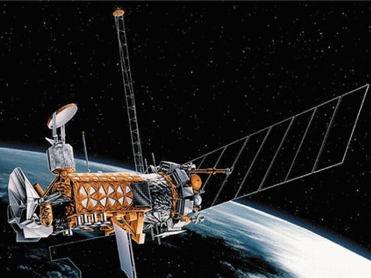
The Defence Meteorological Satellite Program (DMSP) is a long-term meteorological program of the United States Department of Defence (DoD) and the National Oceanic and Atmospheric Administration (NOAA), managed by the United States Air Force (USAF). With 19 satellites in the program, of which 16 are retired, DMSP aims to provide strategic and tactical weather prediction to aid the US military in planning operations at sea, on land and in the air. The program began with the launch of DMSP F-1 in 1976, which is no longer operational, while the latest satellite launch was DMSP F-19 in 2014, which was retired in 2016 due to a power failure. There are three satellites currently operational in the series, DMSP F-16, DMSP, F-17, and DMSP F-18.
Quick facts
Overview
| Mission type | EO |
| Agency | NOAA, USSF, USAF |
| Mission status | Operational (extended) |
| Launch date | 18 Nov 1983 |
| Measurement domain | Atmosphere, Ocean, Land, Gravity and Magnetic Fields, Snow & Ice |
| Measurement category | Cloud type, amount and cloud top temperature, Liquid water and precipitation rate, Atmospheric Temperature Fields, Cloud particle properties and profile, Gravity, Magnetic and Geodynamic measurements, Atmospheric Humidity Fields, Soil moisture, Snow cover, edge and depth, Ocean surface winds |
| Measurement detailed | Cloud top height, Cloud cover, Precipitation intensity at the surface (liquid or solid), Cloud type, Cloud base height, Cloud liquid water (column/profile), Magnetic field (scalar), Magnetic field (vector), Atmospheric specific humidity (column/profile), Atmospheric temperature (column/profile), Snow cover, Soil moisture at the surface, Wind speed over sea surface (horizontal), Snow water equivalent, Ion Density, Drift Velocity, and Temperature, Auroral Emissions, Total electron content (TEC) |
| Instruments | SSJ/5, SSULI, SSM, SSM/T-2, SSM/T-1, SSB/X-2, SSB/X, SSUSI, SSI/ES-3, SSI/ES-2, OLS, SSJ/4, SSM/IS, SSM/I |
| Instrument type | Imaging multi-spectral radiometers (vis/IR), Space environment, Magnetic field, Imaging multi-spectral radiometers (passive microwave), Atmospheric temperature and humidity sounders |
| CEOS EO Handbook | See DMSP (Defense Meteorological Satellite Program) Block 5D summary |
Summary
Mission Capabilities
The DMSP satellites were developed in blocks of identical satellites with the latest being DMSP Block 5D-3 which consists of satellites ranging from DMSP F-15 through to DMSP F-19. DMSP Block 5D-3 satellites each carry six sensors to provide atmospheric, gravitational, land, and snow and ice measurements on a daily basis. The Operational Linescan System (OLS) is a multi-spectral radiometer which monitors the global distribution of clouds and cloud top temperatures twice each day while the Special Sensor Microwave Imager Sounder (SSM/IS) is a multi-purpose imaging microwave radiometer which measures the thermal microwave radiation of the earth, with applications in global measurements of air temperature profiles, humidity profiles and other atmospheric measurements.
For the measurement of gravitational, magnetic and geodynamic parameters, the Special Sensor Ionospheric Plasma Drift / Scintillation Meter (SSI/ES-3) measures the ambient electron density and temperature while the Special Sensor Magnetometer (SSM) measures geomagnetic fluctuations associated with solar geophysical phenomena. The Special Sensor Ultraviolet Limb Imager (SSULI) measures vertical profiles from the natural airglow radiation from atoms, molecules and ions in the upper atmosphere and ionosphere.The Special Sensor Ultraviolet Spectrographic Imager (SSUSI) monitors the composition of the upper atmosphere and ionosphere with spectrographic imagery and photometry.
Performance Specifications
The two instruments on DMSP Block 5D-3 that are most relevant to Earth observation are OLS and SSM/IS. OLS uses a whisk-broom type radiometer that measures in three bands in the visible (VIS) and thermal infrared (TIR) ranges. OLS is able to measure at a spatial resolution of 560 metres in fine mode and 2.7 km in smooth mode along a 300 km scan. SSM/IS is a sounding radiometer that measures across the microwave range from 19-184 GHz in 24 channels. Its spatial resolution varies with the frequency with the highest spatial resolution of 25 km x 17 km and the lowest at 70 km x 42 km at a swath width of 1700 km.
The operational DMSP satellites, F-16, F-17, and F-18, are in sun-synchronous orbits at altitudes ranging between 833 km and 850 km, and orbital inclinations of 98.7°. The orbital period of these satellites is 101 minutes.
Space and Hardware Components
The DMSP satellites were built under a USAF contract by Lockheed Martin Space Systems Company (LMSSC). The spacecraft bus structure was increased in length from 6.7 m to 7.3 m and the mass of the satellites rose to 1220 kg for the Block 5D-3 satellites. The spacecraft is powered by a deployable sun-tracking solar array of size 9.29 m2 which provides 2.2 kW of power. The spacecraft is controlled by a combination flywheel and magnetic control coil system so that sensors are maintained in the desired Earth-looking mode.
DMSP F-19 was retired due to a power failure in 2016. DMSP F-20 was scrapped after the failure of DMSP F-19 as the US congress limited the funds for its launch.
DMSP Block 5D-3 Satellite Series
Spacecraft Launch Mission Status Sensor Complement Ground Segment History of DMSP References
DMSP (Defense Meteorological Satellite Program) is a long-term operational meteorological program of the US DoD (Department of Defense), managed by the USAF and operated by the 6th Satellite Operations Group at Offutt AFB (Air Force Base), Nebraska. The program originated in the early 1960s with the objective to collect and disseminate worldwide cloud cover data on a daily basis (along with oceanographic and solar-geophysical environment parameters). The DMSP system is being used for strategic and tactical weather prediction to aid the US military in planning operations at sea, on land and in the air.
The early DMSP history 1)
In the early 1960s, the reconnaissance community initiated a program using low-altitude satellites as an interim measure to collect cloud-cover data. The highly classified system, known as Program 417, was to support the operational needs of the Corona satellites, designed to provide photo imagery of the Soviet Union. Corona satellites used conventional film to record their data, and the film canisters were jettisoned and returned to Earth via parachute and recovered by aircraft. The DOD wanted to maximize the usefulness of the film and needed a satellite program to predict cloud cover. Thus began Block 1 of DMSP. The program initially involved a small number of Aerospace scientists and engineers in the Electronics Research and Space Physics Laboratories. Their tasks involved improving elements of the primary sensor and developing secondary sensor concepts as well as general science and technology support. Secondary sensors developed in the laboratories flew on numerous DMSP missions and were, in many ways, precursors of the secondary sensor complement now flying on DMSP.
The first DMSP satellites employed a simple spin-stabilized design. They carried a video camera with a 1.27 cm aperture sensing in the 0.2–5 µm regime and two IR systems—the medium-resolution “C” system with 16 channels from 5 to 30 µm, and the high-resolution radiometer working in the 7–14 µm domain. A set of horizon sensors were also used for attitude control and for triggering the camera shutter each time it turned to face Earth. Through the 1960s and into the 1970s, a total of 34 DMSPs were launched, all flying the simple rudimentary payloads. It was not until the design of the Block 5 satellites that more instrument capability began to emerge.
See more information of the early DMSP program in the last chapter of this file.
The DMSP Block 5 series experienced several generations of satellites and instruments (see Table 1). The USAF maintains an operational constellation of two near-polar, sun-synchronous satellites. 2)
In the timeframe 1965 to 2006 (F-17 inclusive), a total of 44 DMSP spacecraft have been launched successfully by the USAF, all were built by Lockheed Martin Corporation.
The Block 5B/C satellites launched between 1971 and 1976 offered increased instrument capability. The vidicon camera was replaced by a constant-speed rotary-scan radiometer. Spin stabilization was abandoned; instead, instruments were mounted on a platform that kept a constant angle between the direction of motion and Earth.
OLS (Optical Linescan System): First flown in 1976, the OLS provided global cloud-cover imagery to military weather forecasters. The OLS operated at two resolutions in the visible spectrum: smooth (2.77 km) and fine (0.55 km). Smooth data processing onboard the spacecraft decreased the resolution and data rate by a factor of 25. The visible channel could detect smoke and dust storms—information that can be critical to strategic planning—as well as ice cover. The instrument was unique in being sensitive enough to view clouds by moonlight. The low-light sensing capability could capture city lights and distinguish lights from fires. This feature could support battlefield damage assessment by enabling commanders to compare the light in a specific area before and after a strike. Thermal IR viewing enabled nighttime cloud viewing at a lower resolution than daytime visible fine-mode data, but provided mission planners with critical 24-hour information about cloud cover and weather conditions.
S/C Bus | S/C Series | Launch Date/ | Sensor Complement | S/C Mass (kg) |
Block 5B | F-1 | 14.10.1971 | Also known as Ops-4311 and P35-26 | 195 |
F-2 | 24.3.1972 | Also known as Ops-5058 | 195 | |
F-3 | 9.11.1972 | Also known as Ops-7323 | 195 | |
F-4 | 17.8.1973 | Also known as Ops-8364 | 195 | |
F-5 | 16.3.1974 | Also known as Ops-8579 | 195 | |
F-6 | 9.8.1974 | Also known as Ops-6983 | 195 | |
Block 5C | F-7 | 24.5.1975 | Also known as Ops-6226 | 194 |
F-8 | 19.2.1976 | Also known as Ops-5140; failed to achieve correct orbit | 175 | |
Block 5D-1 | F-1 | 11.9.1976 / 17.9.1979 | OLS, SSH, SSJ/3, SSB, Contamination Monitor | 450 |
F-2 | 4.6.1977 / 19.3.1978 | OLS, SSH, SSJ/3, SSB, SSB/0, IFM, SSI/E, SSI/P | 450 | |
F-3 | 30.4.1978 / Dec. 1979 | OLS, SSH, SSJ/3, SSB, GFE-3R | 513 | |
F-4 | 6.6.1979 / 29.8.1980 | OLS, SSH, SSJ/3, SSI/E, SSM/T, SSC, SSD | 513 | |
F-5 | 14.7.1980 (failed) | OLS, SSH-2, SSJ/3, SSI/E, SSB/O, SSR | 513 | |
Block 5D-2 | F-6 | 20.12.1982 / 24.8.1987 | OLS, SSH-2, SSI/E, SSJ/4, SSB/A | 750 |
F-7 | 18.12.1983/17.10.1987 | OLS, SSM/T, SSI/E, SSJ/4, SSB, SSJ*, SSM | 750 | |
F-8 | 18.6.1987 / 13.8.1991 | OLS, SSM/I, SSM/T, SSI/ES, SSJ/4, SSB/X-M | 750 | |
F-9 | 3.2.1988 | OLS, SSM/T, SSI/ES, SSJ/4, SSK | 750 | |
F-10 | 1.12.1990 /2. 1995 | OLS, SSM/I, SSM/T, SSI/ES, SSJ/4, SSB/X-2 | 750 | |
F-11 | 28.11.1991 / 8. 2000 | OLS, SSM/I, SSM/T,SSM/T-2,SSJ/4,SSI/ES-2, SSB/X-2 | 830 | |
F-12 | 29.8.1994 | OLS, SSM/I, SSM/T, SSM/T-2, SSJ/4, SSI/ES-2, SSB/X-2, SSM | 830 | |
F-13 | 24.3.1995 | OLS, SSM/I, SSM/T, SSJ/4, SSI/ES-2, SSB/X-2, SSM, SSZ, | 750 | |
F-14 | 4.4.1997 | OLS, SSM/I, SSM/T, SSM/T-2, SSJ/4, SSI/ES-2, SSM, | 750 | |
Block 5D-3 | F-15 | 12.12.1999 | OLS, SSM/I, SSJ/4, SSI/ES-2, SSM-Boom, SSZ | 1220 |
F-16 | 18.10. 2003 | OLS, SSMIS, SSI/ES-3, SSJ5, SSM-Boom, SSULI, SSUSI, SSF, | 1220 | |
F-17 | 04.11.2006 | OLS, SSMIS, SSI/ES-3, SSJ5, SSM-Boom, SSULI, SSUSI, SSF, | 1220 | |
F-18 | 18.10.2009 | OLS, SSMIS, SSI/ES-3, SSJ5, SSM-Boom, SSULI, SSUSI, SSF, | 1220 | |
F-19 | 03.04.2014 | OLS, SSMIS, SSI/ES-3, SSJ5, SSM-Boom, SSULI, SSUSI, SSF, | 1220 | |
S-20 | Due to no launch funds by | OLS, SSMIS, SSI/ES-3, SSJ5, SSM-Boom, SSULI, SSUSI, SSF, | 1220 |
Nomenclature: The DMSP satellites are known as F-xx after launch. Prior to launch, they are designated by S-xx. The 5D-2 series of satellites encompasses F-6 through F-14, while the 5D-3 series of spacecraft begins with F-15. As polar-orbiting spacecraft, all DMSP satellites are being launched from VAFB (Vandenberg Air Force Base), Vandenberg, CA, USA.
DMSP and NOAA-POES Programs Merge
For a period of over 30 years, the DMSP program of the US military, with its LEO polar orbiting satellites (830 km altitude), was in fact a full parallel system to the NOAA-POES series, the US civil LEO weather satellite program in polar orbit. 3) 4) 5) 6) 7)
In the fall of 1993, the US National Performance Review (NPR) and the subsequent Presidential Decision Directive/NSTC-2 (May 5, 1994) called on DOC, DoD and NASA, to “converge” the US civil and military operational meteorological satellite programs (POES of NOAA and DMSP of DoD), in order to reduce duplication of effort and to generate cost savings. In October 1994, an Integrated Program Office (IPO), consisting of a team made up of NOAA, NASA and DoD representatives, was established organizationally under NOAA (with the IPO Headquarters located in Silver Spring, MD) with the explicit objective to integrate their separate meteorological programs into a single program that includes: planning, development, management, acquisition, and operations. A tri-agency MOA (Memorandum of Agreement) was signed in May 1995. The merged program received the name of NPOESS (National Polar-orbiting Operational Environmental Satellite System). The IPO is a tri-agency office reporting through NOAA to an Executive Committee of representatives from DOC, DoD and NASA.
In May 1998, the US Air Force Space Command transferred its day-to-day operations of the DMSP spacecraft to NOAA. With this action, NOAA assumed full responsibility for the operation of both the POES and DMSP satellite constellations. NOAA maintains and conducts joint satellite control operations at a collocated operations center where it also conducts operations of NOAA's GOES (Geostationary Operational Environmental Satellite) series (from Suitland, MD).
The DoD DMSP program and the POES program convergence takes place in two phases.
• First phase: Starting in May 1998, all DMSP satellite operational command and control functions of AFSPC (Air Force Space Command) were transferred to a tri-agency Integrated Program Office (IPO) established within NOAA. NOAA was given the sole responsibility of operating both satellites programs, POES and DMSP (from NESDIS, Suitland, MD).
• During the second phase, the IPO will launch and operate the new NPOESS satellites (starting in 2009) that will satisfy both the DoD and Department of Commerce (DOC/NOAA) requirements.
DMSP and NOAA Polar Programs Separate Again
In Feb. 2010, the NPOESS (National Polar-orbiting Environmental Satellite System) tri-agency program was terminated by the US government due to severe cost overruns and program delays. The NPOESS program was a joint DoD/NOAA/NASA endeavor that tried to integrate the capabilities and infrastructure of the NOAA POES (Polar-Orbiting Environmental Satellite) program, the DoD DMSP (Defense Meteorological Satellite Program), and NASA’s long-term continuous climate record collection. - The President's FY 2011 budget request for NOAA directed the NPOESS program to split into separate NOAA/NASA and DoD programs.
The major challenge of NPOESS was jointly executing the program between three agencies of different size with divergent objectives and different acquisition procedures.
In 2009, an IRT (Independent Review Team) concluded that the current NPOESS program, in the absence of managerial and funding adjustments, has a low probability of success and data continuity is at extreme risk. The Office of Science and Technology, with the Office of Management and Budget and the National Security Council, as well as representatives from each agency, examined various options to increase the probability of success and reduce the risk to data continuity. 8) 9)
NOAA's restructured satellite program, the civilian JPSS (Joint Polar Satellite System), was created in the aftermath of the White House's Feb. 2010 decision to cancel NPOESS. The development of the new JPSS will be managed by NASA/GSFC while the spacecraft will be owned and operated by NOAA. The launch of JPSS-1 is planned for 2016.
NOAA, through NASA as its acquisition agent, will procure the afternoon orbit assets that support its civil weather and climate requirements and DoD will independently procure assets for the morning orbit military mission - referred to as DWSS (Defense Weather Satellite System). Both agencies will continue to share environmental measurements made by the system and support the operations of a shared common ground system.
The Administration decision for the restructured Joint Polar Satellite System will continue the development of critical Earth observing instruments required for improving weather forecasts, climate monitoring, and warning lead times of severe storms. NASA’s role in the restructured program will be modeled after the procurement structure of the successful POES (Polar Operational Environmental Satellite) and GOES (Geostationary Operational Environmental Satellite) programs, where NASA and NOAA have a long and effective partnership. The partner agencies are committed to maintaining collaborations towards the goal of continuity of earth observations from space.
The restructured JPSS (Joint Polar Satellite System) is planned to provide launch readiness capability in FY 2015 and FY 2018 (with launches of JPSS-1 in 2016 and JPSS-2 in 2019, respectively) in order to minimize any potential loss of continuity of data for the afternoon orbit in the event of an on orbit or launch failure of other components in the system. Final readiness dates will not be baselined until all transition activities are completed. 10)
The following restructured concept scenario emerged in 2010:
• NOAA/NASA Joint Polar Satellite System (JPSS) covers the afternoon (13:30 hours) orbit
• JPSS flies an “NPP-like” satellite bus
• DoD covers the early morning (05:30 hours) orbit. A DMSP Follow-on program (beyond DMSP-F-20) is in planning.
• NOAA manages the JPSS ground system.
The European polar weather satellite program of EUMETSAT, namely the MetOp series, is also involved in this new overall scenario through the EPS (EUMETSAT Polar System) agreements (Figure 2).
Space Segment of Block 5D-3 Series
The DMSP satellites were built under a USAF contract by LMSSC (Lockheed Martin Space Systems Company), Sunnyvale, CA. They are three-axis stabilized. Pointing of the satellites is maintained by three orthogonal reaction wheel assemblies. A precision mounting platform provides a pointing accuracy of 0.01º. The spacecraft bus structure was increased in lengthfrom 6.7 m to ~7.3 m and the mass of the satellite rose to ~1220 kg. The spacecraft is separated into four sections or modules: 11) 12)
• A precision mounting platform for sensors and equipment requiring precise alignment
• An equipment support module containing the electronics, reaction wheels, and some meteorological sensors
• A reaction control equipment support structure containing the third-stage rocket motor and supporting the ascent phase reaction control equipment
• A deployable sun-tracking solar array of size 9.29 m2 (10 panels), spacecraft power of 2.2 kW.
The spacecraft stabilization is controlled by a combination flywheel and magnetic control coil system so that sensors are maintained in the desired earth-looking mode. One feature is the precision-pointing accuracy of the primary imager to 0.01º provided by a star sensor and an updated ephemeris navigation system. This allows automatic geographical mapping of the digital imagery to the nearest picture element. The Block 5D-3 series spacecraft have a design life of 5 years.
The F-15 and F-16 DMSP satellites are Block 5D-3 series that accommodate larger and more advanced sensor payloads than earlier generations. They also feature a more advanced attitude control system for precision pointing; a more powerful onboard computer with increased memory - allowing greater spacecraft autonomy; a higher rate command link for shorter ground contact times; an increased battery capacity that prolongs the mission duration, and an improved onboard autonomy (60 days). The F-16 spacecraft is in fact the first full Block 5D-3 satellite. Although the F-15 spacecraft features the new Block 5D-3 bus, it is flying the legacy 5D-2 sensor complement.
Orbital Parameters of DMSP: 13)
Sun-synchronous orbits, altitude = 811 - 853 km (833 km nominal), inclination = 98.9º, period = 101.6 minutes, there are normally two satellites in operation at any one time (one in a morning and one in a late morning equatorial crossing time).
RF communications: DMSP downlinks mission data stored onboard Stored Mission Data (SMD) once per orbit and has two real-time data transmissions, the Real-time Data Smooth (RDS) and Real Time Data fine (RTD).
Onboard preprocessing of data by the OLS sensor system provides for the various modes of data output. OLS data consists of both visual or Light data (L data) and infrared or Thermal (T data) modes. Infrared Fine resolution data (TF data) can be collected continuously, day and night. Visible fine (LF data) is collected during daytime only. Storage capacity and transmission constraints limit the quantity of fine resolution data (LF or TF) which can be provided in the SDF (Stored Data, Fine) mode. Data smoothing permits global coverage in both the infrared (TS) and visible (LS) spectrum to be stored on the primary tape recorders in the SDS (Stored Data Smoothed) mode.
The data rate is 1.33 MBit/s for SDF (TF or LF) or 2.66 Mbit/s if SDS is interleaved bit-by-bit (TF/LF or TS/LS). The DMSP RTS Mux accepts either data rate and formats Equipment Status Telemetry data with the incoming stored data stream. This 3.072 Mbit/s data stream is then transmitted via a DOMSAT communications satellite link to AFWA (Air Force Weather Agency) and FNMOC (Fleet Numerical Meteorology and Oceanography Center) for processing.
DMSP transmits two S-band downlinks in real-time: Real Time Data (RTD) link containing OLS fine (TF/LS or LF/TS) data; and Real Time Smooth (RDS) data stream containing OLS smooth data. - The F-16 spacecraft features a dedicated S-band for RTD at a frequency of 2222.5 MHz. The date rate of the RDS increases to 88.75 kbit/s unencoded (177.5 kbit/s encoded). Additionally, there is the capability to transmit a UHF RDS transmission at 400.328 MHz and at 400.822 MHz. All DMSP downlinks are encrypted.
Launch
The first of six new DMSP 5D-3 spacecraft was scheduled to be delivered to the Air Force in June 1990. Following the loss of the Space Shuttle Challenger in January 1986, however, all of them were rescheduled for launch atop modified Titan-II intercontinental ballistic missiles.
• The DMSP Block 5D-3-1 was launched on December 12, 1999 from VAFB, CA on a Titan-2 vehicle with 6 Block 5D-2 instruments to test the new satellite bus (F15 on orbit) followed by the F16 satellite on October 18, 2003 with the new 5D-3 payload. Since F16, all 5D-3 satellites have been carrying the same payloads.
• On Nov. 4, 2006, the DMSP F-17 spacecraft was launched on a Delta-4 (EELV) rocket from VAFB (launch mass of 1154 kg).
• On October 18, 2009, the DMSP F-18 spacecraft was launched on an Atlas-5 rocket of ULA from VAFB (launch mass of 1230 kg)
• On April 3, 2014, the DMSP F-19 spacecraft, built by Lockheed Martin, was successfully launched from Vandenberg Air Force Base, CA, on an Atlas-5 vehicle. DMSP-19 joins six other satellites in polar orbit providing weather information.
- Several features on DMSP-19 improve reliability and performance. Those include a more capable power subsystem, an upgraded on-board computer and better battery capacity that extends mission life. Additionally, the satellite carries a new attitude control subsystem and a star tracker. The current Block 5D series also accommodates larger sensor payloads than earlier generations. 14)
Operational Status and Imagery of the DMSP Series
• March 23, 2022: Arctic sea ice appeared to reach its annual maximum extent on February 25, 2022, after growing through the fall and winter. This year’s wintertime extent is the tenth lowest in the satellite record maintained by the National Snow and Ice Data Center. It also tied 2015 as the third earliest maximum on record. 15)
- Arctic sea ice extent peaked at 14.88 million km2 (5.75 million square miles), a total area that is roughly 770,000 km2 (297,300 square miles) below the 1981–2010 average maximum. Compared to the average maximum, the Arctic Ocean in 2022 is missing an area of ice equivalent to the states of Texas and Maine combined.
- Every year, the cap of frozen seawater floating on top of the Arctic Ocean and neighboring seas melts during the spring and summer and grows in the fall and winter. That ice reaches its maximum extent around March after growing through months of cold winter darkness; it shrinks to its minimum extent in September. In the Southern Hemisphere, Antarctic sea ice follows an opposite cycle.
- To estimate sea ice extent, satellite sensors gather data that are processed into daily images, with each image grid cell spanning an area of roughly 25 km by 25 km (15 miles by 15 miles). Scientists then use these images to estimate the extent of the ocean where sea ice covers at least 15 percent of the water. The graph above shows Arctic daily sea ice extent in 2022, 2021, and 2012 compared to the 1981–2010 average.
- Since satellites began reliably tracking sea ice in 1979, maximum extents in the Arctic have declined by roughly 13 percent per decade, with minimum extents declining about 2.7 percent per decade. These trends are linked to warming caused by human activities, such as emissions of heat-trapping carbon dioxide. Other NASA analyses show that the Arctic is warming about three times faster than other regions of Earth.
• September 16, 2021: Sea ice in the Arctic Ocean and neighboring basins appears to have hit its annual minimum extent on September 16, 2021, after waning in the spring and summer. The summertime extent is the twelfth lowest in the satellite record, according to scientists at the National Snow and Ice Data Center and NASA. 16)
- Less sea ice melted in 2021 even as the planet as a whole was warmer than usual—with new temperature records in North America and Eurasia, drought in the U.S. West, and episodes of intense melting on Greenland’s ice sheet. But farther north, conditions stayed generally cool and stormy across the Arctic Ocean. For much of the summer, low pressure over the Arctic brought cloudy skies, which limits the amount of sunlight that can reach the ice and spur melting. Storms can also spread the ice out, slowing the decline of its extent.
- Such differences from place-to-place and year-to-year are to be expected. “I don’t see any inconsistency with the Arctic sea ice extent not breaking any records this year despite global temperatures being high,” said Claire Parkinson, a sea ice scientist at NASA’s Goddard Space Flight Center. “The key is that the Earth is large and there are differences regionally.”
- “We don’t expect sea ice to be lower every year,” added Walt Meier, a sea ice researcher at the National Snow and Ice Data Center, “just like we don’t expect temperatures to be warmer everywhere on Earth every year even with global warming.”
- Long-term trends are more important than any single year, and those trends are still pointing strongly downward. The 15 lowest minimum extents in the 43-year satellite record have all occurred in the past 15 years (2007 to 2021).
- Sea ice is also trending younger and thinner; that is, there is less multi-year ice that survives a summer season and thickens over the subsequent winter. According to Meier, data show that sea ice this summer contained the second-lowest amount of multi-year ice on record.
- Parkinson and Meier think that this summer, plenty of ice was close to disappearing but never quite reached that point—maintaining extent but not thickness. “There does appear to be a fair amount of ice in the Beaufort and Chukchi Seas that seems to have gotten quite thin,” Meier said, “but there just wasn’t quite enough energy through the summer to melt it out completely.”
• April 19, 2021: The amount of sea ice around Earth’s poles waxes and wanes with the seasons, melting through spring and summer and growing through fall and winter. In recent decades, there has been more waning than waxing, as polar sea ice has mostly been in a long-term decline since the start of the satellite record in the 1970s. The maps on this page represent the most recent snapshots of those annual highs and lows. 17)
- “The 2020-2021 Arctic data further confirm that the Arctic sea ice coverage is well below what it had been in the 1970s and 1980s,” said Claire Parkinson, a sea ice scientist at NASA’s Goddard Space Flight Center. “The 2020–2021 Antarctic data reveal an ice cover that has rebounded somewhat from its 2017 record low but is nowhere close to growing back to its much greater 2014 ice coverage.”
- When Arctic sea ice reached its minimum extent on September 15, 2020, it spanned just 3.74 million km2 (1.44 million square miles)—the second-lowest minimum since the start of the satellite record in 1979. In recent decades, Arctic melting seasons have been growing longer and much of the older, thicker ice has been lost.
- Some Arctic marginal seas fared worse than others. In the Labrador Sea, sparse sea ice cover during the winter posed challenges for Inuit people, disrupting some ice highways that connect communities in the region. In the Gulf of Saint Lawrence, the lack of sea ice led seal pups to cluster onshore, where they were more vulnerable to predators.
- Sea ice around Antarctica has been variable lately. Since the start of the satellite record in the late 1970s, seasonal ice cover increased gradually and peaked at a record high in 2014. The next few years showed a rapid decline, wiping out decades of increases. There have been small rebounds in recent years, but nowhere near the record high.
- To see these maps in context with the longer-term changes, visit our World of Change series for Arctic sea ice and for Antarctic sea ice.
• January 6, 2021: Throughout 2020, the Arctic Ocean and surrounding seas endured several notable weather and climate events. In spring, a persistent heatwave over Siberia provoked the rapid melting of sea ice in the East Siberian and Laptev Seas. By the end of summer, Arctic Ocean ice cover melted back to the second-lowest minimum extent on record. In autumn, the annual freeze-up of sea ice got off to a late and sluggish start. 18)
- But any single month, season, or even year, is just a snapshot in time. The long view is more telling, and it is troubling.
- The change is part of a cycle called the “ice-albedo feedback.” Open ocean water absorbs 90 percent of the Sun’s energy that falls on it; bright sea ice reflects 80 percent of it. With greater areas of the Arctic Ocean exposed to solar energy early in the season, more heat can be absorbed—a pattern that reinforces melting. Until that heat escapes to the atmosphere, sea ice cannot not regrow.
- Dominated by thin first-year ice, along with some older ice thinned by warm ocean water, the Arctic sea ice pack is becoming more fragile. In summer 2020, ships easily navigated the Northern Sea Route in ice-free waters, and even made it to the North Pole without much resistance.
- Fortunately, summers are still not entirely ice-free. “We’ve been hovering for some time around 4 million square kilometers of Arctic sea ice each summer,” said Stroeve, a researcher at University of Manitoba. She added that she intends to examine which conditions and processes could push sea ice to the next “precipitous drop”—when the extent of summer ice cover drops to a new benchmark of 3 million km2.
• December 9, 2020: After the spring and summer melt season, the cap of frozen seawater floating on top of the Arctic Ocean begins to refreeze. In 2020, however, the annual freeze has been unusually slow. 19)
- When Arctic sea ice reached its annual minimum in September 2020, it was one of the lowest extents of the satellite record—second only to the record low in September 2012. But unlike 2012, the ocean did not see its typical rate of refreezing in 2020. As a result, the sea ice extent for this October was the lowest on record for any October. Ice growth picked up the pace at the start of November but then slowed again, leaving plenty of open water in the Barents and Kara seas at the start of December.
- According to the National Snow & Ice Data Center (NSIDC), October 2020 was “the largest departure from average conditions seen in any month thus far in the satellite record.” Scientists have used satellites to continuously measure sea ice since 1979. The chart above shows how the extent of sea ice has progressed in 2020. For context, ice extents for 2012 (the record low extent) and 2016 (another year with a slow refreeze) are also charted.
- Regional variations in water temperatures and weather can affect the amount of sea ice in different parts of the Arctic. In 2020, ocean currents helped flush ice out from the Russian Arctic coast. An intense summer storm also parked over the Arctic Ocean, similar to the storm that contributed to the record low sea ice minimum in 2012.
- But it was the early ice retreat amid warm Arctic air temperatures that set the stage for the slow freeze-up in 2020. Starting in May, warm air over Siberia provoked rapid melting in the East Siberian and Laptev Seas. With large expanses of dark, ice-free water exposed to the warming sunlight, the ocean could gain more heat than usual over the course of the summer, which reinforced melting. Until that heat escaped to the atmosphere, sea ice could not reform.
• September 23, 2020: The Arctic sea ice extent continues its long-term downward trend. According to researchers at NASA and the National Snow and Ice Data Center (NSIDC) the Arctic sea ice likely reached its annual minimum extent on September 15, 2020. 20)
- Analyses of satellite data showed that the Arctic ice cap shrank to 3.74 million km2 (1.44 million square miles), making it the second-lowest minimum on record. Experts cautioned that the announcement is preliminary, and there is still a possibility that changing winds or late season melting could push the ice extent lower.
- Numerous factors combined to shrink sea ice so much in 2020. In spring, a heatwave across Siberia set the stage for rapid early season melting. Also, sea ice was already much thinner going into the 2020 melt season than in years past—the accumulated result of the general long-term decline in summer sea ice extent. And scientists think warm water could be working its way under the ice and melting it from below.
- Weather can also affect the amount of ice across the Arctic. From late July into early August, scientists watched an atmospheric low-pressure system spin over the Arctic Ocean and wondered how it would affect the ice. A similar storm in 2012 was a major cause of the lowest sea ice minimum on record. “The summer 2020 storm definitely had an effect, but it didn’t seem sufficient to cause the really significant loss of ice to drive a new record low,” Petty said.
- In any given year, there are regional variations in air temperatures, water temperatures, and weather that promote or inhibit melting in different parts of the Arctic. By the date of the 2020 minimum, there was still more sea ice remaining in the Beaufort Sea compared to 2012, and slightly less in the Laptev and East Greenland seas.
• March 25 2020: The 2019-2020 winter was warm for most of the middle latitudes of the Northern Hemisphere. Not so in the Arctic, where persistent cold air helped sea ice grow to a larger extent than in several recent years. Still, there was not enough growth during the fall and winter months to bring sea ice back to long-term average levels. 21)
- “So far this year the Arctic sea ice has been more extensive than in most years of the past decade, but it is not close to as extensive as it typically was in the 1980s and 1990s,” said Claire Parkinson, a sea ice scientist at NASA’s Goddard Space Flight Center in Greenbelt, Maryland. “Recovery to 1980s levels would take thickening of the ice, as well as a greater expanse.”
- Every year, the cap of frozen seawater floating on top of the Arctic Ocean and neighboring seas melts during the spring and summer and grows in the fall and winter. The ice reaches its annual maximum extent sometime between February and April. In 2020, sea ice reached its annual maximum extent on March 5, when satellites observed it spread across 15.05 million km2 (5.81 million square miles).
- Jennifer Francis, a scientist from the Woods Hole Research Center who studies the changing Arctic, noted that there can be great variability from year to year because of fluctuations in weather and ocean currents. This year, a strong stratospheric polar vortex helped trap cold air in the Arctic. The same phenomenon left mid-latitudes warmer and generally less snowy than normal.
- “This winter happened to have an upswing in the ice cover, but it’s still well below normal and there’s every reason to expect the downward trend will continue,” Francis said. The downward trend is clear when you chart successive seasonal ups and downs as measured by satellites over four decades: the annual maximums and minimums are generally becoming smaller over time. This change, while seemingly remote and regional, has global consequences.
- What happens in the Arctic doesn’t stay in the Arctic,” Francis said. “Losing so much bright, white ice means the Earth now absorbs much more of the Sun’s energy, rather than reflecting it back to space. This amplifies the warming effect of increasing greenhouse gases by 25 to 40 percent.”
- On the other side of the planet, the opposite seasonal cycle just concluded with the end of summer. Sea ice around Antarctica reached its annual minimum extent on February 20-21, 2020.
- “The Antarctic sea ice coverage continues the small rebound that it has experienced since its precipitous decline from 2014 to 2017,” Parkinson said, “although it is nowhere close to rebounding to its record high 2014 expanse.”
• February 4, 2020: A polar bear’s life seems simple enough: eat seals, mate, and raise cubs. But a recent study shows some subpopulations of polar bears are struggling to complete these essential tasks because of declining concentrations of Arctic sea ice. 22)
- The Arctic sea ice cap is a large area of frozen seawater floating on top of the Arctic Ocean and its surrounding seas and straits. For polar bears, the sea ice is a crucial platform for life. They use the ice to travel long distances to new areas. They hunt for seals by finding their dens or sitting next to gaps in the ice, waiting for the unsuspecting prey to pop up. Sometimes, pregnant females dig in the sea ice to create maternity dens, where they give birth and take care of their cubs.
- In recent decades though, this critical habitat has been shrinking. Sea ice concentrations have declined by 13 percent each decade since 1979 due to increasing global temperatures. Arctic regions have warmed twice as fast as the rest of the world, so seasonal sea ice is also forming later in the fall and breaking up earlier in the spring.
- “We know that sea ice, which is where the bears need to be, is decreasing very rapidly,” said Kristin Laidre, an Arctic ecologist at the University of Washington. “When there’s no sea ice platform, the bears end up moving onto land with no or minimal access to food. Our research looked at how these changes affect their body condition and reproduction.”
- In a new study published in Ecological Applications, Laidre and her colleagues described how declining sea ice concentrations are affecting the behavior, health, and reproductive success of polar bears. Using field observations and remote sensing, the study showed that polar bears are spending more time on land and are fasting for longer periods of time. Mother bears are also producing smaller cub litters, which the team projected will continue to decline for the next three polar bear generations. 23)
- “Climate-induced changes in the Arctic are affecting polar bears,” said Laidre, who was the main author of the study. “They are an icon of climate change, but they’re also an early indicator of climate change because they are so dependent on sea ice.”
- The study team found that most bears follow the seasonal growth and recession of sea ice to end up on Baffin Island in the fall, when sea ice is usually at its lowest extent. They usually wait on Baffin Island until the ice forms again so they can leave. On average, the bears are spending 30 more days on land now than they did in the 1990s. Laidre says that is because the ice is retreating earlier and there has been more open water in recent summers.
- “That’s important because when the bears are on land, they do not hunt seals,” said Laidre. “They have the ability to fast, but if they don’t eat for longer periods, they get thinner. This can affect their overall health and reproductive success.”
- To assess polar bear health, the team quantified the condition of bears by assessing their level of fatness after sedating them or inspecting them visually from the air. Laidre and colleagues classified fatness on a scale of 1 to 5. Results showed the bears’ body condition was linked with sea ice availability in the current and previous year.
- Cub litter size was also affected by the body condition of the mothers and by sea-ice availability. The researchers found larger litter sizes when the mothers were in a good body condition and when spring breakup occurred later in the year, meaning bears had more time on the sea ice in spring to find food.
- Then finally, the team used mathematical models to forecast future reproductive success. The model took into account the relationship between sea-ice availability and the bears’ body fat and variable litter sizes. They projected that the normal cub litter size of two may decrease within the next three polar bear generations (37 years), mainly due to the projected decline of sea ice in the coming decades.
- The results of the study were not necessarily surprising for Laidre, who has been studying the changes in the Arctic ecosystem for the past 20 years. She says it is well known that changes in the climate are having a negative effect on polar bears. Even if greenhouse gases were curbed immediately, sea ice would likely continue to decline for several decades because large-scale changes take a long time to propagate through Earth’s climate system.
- In the meantime, Laidre hopes this study’s information will be used to further understand the impacts of sea ice loss on the species. “Polar bears are a harbinger for the future,” said Laidre. “The changes we document here are going to affect everyone around the globe.”
• September 24, 2019: The long-term trend for Arctic sea ice extent has been definitively downward. Arctic sea ice reached its annual summer minimum on September 18, 2019, according to NASA and the National Snow and Ice Data Center (NSIDC). Analysis of satellite data by NSIDC and NASA showed that the extent of ice cover this year effectively tied 2007 and 2016 as the second lowest in the satellite record, which dates back to late 1978. The sea ice cap shrank to 4.15 million km2 (1.60 million square miles) in 2019. 24)
- The Arctic sea ice cap is an expanse of frozen seawater floating on top of the Arctic Ocean and neighboring seas. Every year it expands and thickens during the fall and winter, then grows smaller and thinner during the spring and summer. But in recent decades, increasing air and water temperatures have caused marked decreases in Arctic sea ice extents in all seasons, with particularly rapid reductions in the summer ice extent.
- Changes in Arctic sea ice cover have wide-ranging impacts. The sea ice affects local ecosystems, regional and global weather patterns, and the circulation of the oceans.
- “This year’s minimum shows that there is no sign that the sea ice cover is rebounding,” said Claire Parkinson, a senior scientist at NASA’s Goddard Space Flight Center. “The long-term trend for the Arctic sea ice extent has been definitively downward.”
- “This was an interesting melt season,” said Walt Meier, a sea ice researcher at NSIDC. The season started with a very low sea ice extent in May, followed by very rapid ice loss in July and the beginning of August. “At the beginning of August, we were at record low ice levels for that time of the year, so a new minimum record low could have been in the offering.”
- Unlike 2012—when a powerful August cyclone smashed the ice cover and accelerated its decline to the lowest ice extent on record — this melt season did not bring any extreme weather events. Although areas within the Arctic Circle saw average temperatures 4 to 5º Celsius above normal, events such as the severe Arctic wildfire season and the European heat wave did not have much impact on sea ice melting.
- “By the time the Siberian fires kicked into high gear in late July, the Sun was already getting low in the Arctic, so the effect of the soot darkening the sea ice surface wasn’t that large,” Meier said. “As for the European heat wave, it definitely affected land ice loss in Greenland and also caused a spike in melt along Greenland’s east coast. But that is an area where sea ice is being transported down the coast and melting fairly quickly anyway.”
• March 9, 2018: Arctic sea ice reaches its maximum extent each March, following months of growth during usually frigid and dark autumn and winter. The date of maximum extent for winter 2018 has yet to be determined, but in February 2018, the average ice extent was the lowest of any February on record. 25)
- The map of Figure 31 shows the average concentration of Arctic sea ice in February 2018. Opaque white areas indicate the greatest concentration, and dark blue areas are open water. All icy areas pictured here had an ice concentration of at least 15 percent (the minimum at which space-based measurements give a reliable measurement), and cover a total area that scientists refer to as the “ice extent.”
- The February extent averaged 13.95 million km2, according to the NSIDC (National Snow & Ice Data Center). That is 1.35 million km2 below the 1981–2010 average for February. The chart of Figure 30 shows how Arctic sea ice growth this year compares with all years since 1979.
- The lackluster ice growth—and the decline in areas such as the Bering and Chukchi seas—was influenced by a so-called “winter warming event.” (Read about the complex chain of events that lead to these events here.) Low pressure off of Greenland and high pressure over Europe helped move warm air masses—and possibly some warm water—from the North Atlantic into the Arctic Ocean. A similar scenario also played out on the Pacific side: low- and high-pressure systems set up in such a way as to move warm air and water from the North Pacific through the Bering Strait.
- “We have seen winter warming events before, but they’re becoming more frequent and more intense,” said Alek Petty, a sea ice researcher at NASA’s Goddard Space Flight Center.
- Areas of unusual warmth are visible in the map of Figure 32, which shows air temperature anomalies for February 2018. Red and orange colors depict areas that were hotter than average; blues were colder than average. At times, the North Pole saw temperatures climb above freezing, soaring 20 to 30 ºC above the norm.
- Notice the area north of Greenland. This is the site of another exceptional event this winter: open water instead of sea ice cover. Without the ice cover here, heat is being released from the ocean to the atmosphere, making the sea ice more vulnerable to further melting. “This is a region where we have the thickest multi-year sea ice and expect it to not be mobile, to be resilient,” Petty said. “But now this ice is moving pretty quickly, pushed by strong southerly winds and probably affected by the warm temperatures, too.”
- NASA’s Operation IceBridge—an airborne mission to map polar ice—will make measurements in the area when annual science flights resume in late March 2018.
• December 20, 2017: With the help of Secretary of the Air Force Heather Wilson, the SMC (Space and Missile Systems Center) has unveiled the final Defense Meteorological Support Program satellite, DMSP-20, for display at the Schriever Space Complex within the Gordon Conference Center. 26) 27)
- "This display represents a nearly 60-year history of environmental monitoring success by a satellite constellation that continues to provide crucial weather information to our nation's leaders, civil users, and warfighters," said Wilson. DMSP got its start in 1961, when the National Reconnaissance Office established a meteorological satellite program to provide information on cloud cover over the Soviet Union for the once highly-classified Corona photographic reconnaissance satellites.
- Retired Air Force Col. Thomas Haig, recently presented with a piece of the DMSP-20 satellite on Aug. 9, was selected to create and manage DMSP.
- Although intended as an interim program, the highly successful DMSP was transferred to the Space Systems Division - forerunner of today's SMC - and launched its first satellite into low earth orbit on Aug. 23, 1962.
- In the intervening six decades, DMSP has had an impressive succession of successes. It provided the earliest tactical uses of spaceborne weather information and the world's first use of satellite imagery to support tactical military operations during the Vietnam conflict. The information DMSP provides has been crucial to the support of military operations ever since, from first Gulf War to real-time situational awareness for current operations in Iraq and Afghanistan.
- "But DMSP supports more than just military operations," explained Lt. Gen. John Thompson, SMC commander and Air Force program executive officer for space. ”NOAA and various other civil and humanitarian organizations use DMSP imagery and data for weather forecasting. This includes numerous missions that rely on data from snow cover and tropical cyclone intensity to cloud temperatures and magnetic fields in space. Even NASA uses DMSP weather information to help plan future launches, as they did with launches stretching back to the Apollo and Space Shuttle programs."
- Although the final DMSP satellite launched in 2014 (DMSP-19), the constellation as a whole will continue to provide data used to create weather forecast models and provide crucial weather information for the foreseeable future.
- This includes DMSP-14, which was launched in 1997 and completed its historic 100,000th orbit around the Earth last summer.
- "The fact that DMSP-14 is providing weather data 17 years past its designed mission life of three years is a testament to the craftsmanship of the satellite and the hard work of the government and contractor teams who continue to make the DMSP program a resounding success," said Dr. Stephen Pluntze, deputy director of SMC's Remote Sensing Systems Directorate and former director of the Defense Weather Systems Directorate.
- The SMC (Space and Missile Systems Center) was responsible for procuring DMSP satellites. The DMSP constellation is operated by a coalition of mission partners including NOAA's Office of Satellite and Product Operations and the 50th Operations Group Detachment 1, both located in Suitland, Maryland.
- Backup command and control operations are conducted by the 6th Space Operations Squadron located at Schriever AFB, Colorado. Lockheed Martin Space Systems designed the spacecraft, and Northrop Grumman worked with the Air Force Research Laboratory to provide the sensors integrated onto the spacecraft.
- SMC, located at Los Angeles Air Force Base in El Segundo, California, is the U.S. Air Force Space Command's center of excellence for acquiring and developing military space systems. SMC's portfolio includes the Global Positioning System, military satellite communications, defense meteorological satellites, space launch enterprise, satellite control networks, remote sensing systems, and space situational awareness capabilities.
• November 8, 2017: For 18 years, a fully-built, ready-to-launch weather satellite sat inside a Lockheed Martin facility near Moffett Field in Sunnyvale, California. Scientists were waiting for the spacecraft to be called into active duty since it was completed during the Clinton administration. 28)
- A different order from Washington arrived instead. Because of resistance in Congress — particularly from Rep. Michael Rogers of Alabama, who chairs a key House Defense subcommittee — Capitol Hill told the Air Force to take the satellite apart.
- Congress simply refused to fund the Air Force's request for $120 million to launch the spacecraft, even though the service said it was needed for weather forecasting, a crucial aspect of battlefield planning. In addition, climate scientists were counting on that satellite to help them monitor Arctic ice melt.
- Now, instead of helping scientists and members of the military, the satellite will go on display — stripped of its expensive instruments — next month in a museum at Los Angeles Air Force Base in El Segundo, California.
- The decision to dismantle the satellite shocked scientists, who were hoping to use a microwave sensor aboard it to help them avoid a dangerous gap in Arctic sea ice data that may open up between now and 2023. That is the estimated year when the next Air Force weather satellite launch is planned.
• August 4, 2017: The DMSP -19 mission will soon cease transmitting weather data after nearly three and a half years of operational service, the U.S. Air Force said. 29)
- There is no impact to the strategic weather mission, and the DMSP constellation remains able to support military requirements through resilient systems and processes, the Air Force reported. The remainder of the constellation continues to provide weather and atmospheric data to users.
- Operators lost the ability to command the satellite Feb. 11, 2016, following a power failure within the command and control system, the Air Force noted. Since that time the satellite has provided tactical data to field units but has not provided full-orbit weather imagery to the 557th Weather Wing, Offutt Air Force Base, Neb., and the U.S. Navy’s Fleet Numerical Meteorology and Oceanography Center, Monterey, CA.
- The DMSP operations team has remained in regular contact with the vehicle and continued to monitor telemetry since the incident, the Air Force said. However, the team acknowledged a loss of attitude control was unavoidable due to the inability to command. Once the satellite loses attitude control it will begin to tumble, causing the power system to deplete and all satellite transmissions to cease. The tumble is predicted to occur late next month. The Joint Space Operations Center will track the satellite and provide conjunction warnings if required.
- DMSP F-19 was launched in April 2014. While space-based weather assets were originally launched and operated by the U.S. Air Force, a 1994 presidential directive realigned primary command and control of DMSP under the Department of Commerce’s National Oceanic and Atmospheric Administration.
• December 16, 2016: As previously reported, the Arctic sea ice cover was lower in November 2016 than any other November in the satellite record. It turns out that the Arctic was not alone. Sea ice at the other pole, around Antarctica, also reached a record November low. 30)
- During this time of year, the Arctic Ocean and neighboring seas are refreezing after the annual summer melt season. Conversely, the sea ice fringing Antarctica is normally melting at this time of year, during the austral spring and summer. What is unusual is the amount of melting so far in the Antarctic, spurred by warm air temperatures and shifting winds.
- The ice extent for November 2016 averaged just 14.54 million km2. The yellow line of Figure 34 shows the median extent from 1981 to 2010, and gives an idea of how conditions this November strayed from the norm. Specifically, the November extent this year was 1.81 million km2 below the 1981 to 2010 average.
- The melt season started early this year, after Antarctic sea ice reached its annual maximum extent on August 31. By November, the ice reached daily record lows amid air temperatures that were 2 to 4 degrees Celsius above average. Winds that usually disperse the ice instead shifted direction and compressed it around various land areas.
- It remains to be seen how much Antarctic sea ice will melt during the remainder of the season; sea ice usually reaches its annual minimum extent in February. In some places around the continent, sea ice can melt completely before starting the annual cycle of refreezing.
- In recent years, notably from 2012 to 2014, the period of refreezing has culminated in record-high maximum extents. On an annual basis, the total Antarctic sea ice extent has increased about 1 percent per decade since 1979. Still, the long-term trend still shows a global decline in sea ice. The chart of global extent demonstrates how, over the long term, the slight increases in Antarctic sea ice have not offset the large losses in the Arctic.
• July 25, 2016: The satellite anomaly resolution team recently closed their investigation into the DMSP-19 anomaly. The anomaly team determined there was a power failure within the command and control system that affected onboard cryptographic equipment. Due to this failure, commands are unable to reach the command processor. Both the A and B side of the command and control subsystem failed, eliminating the possibility of commanding via a back-up command path. The satellite is not repairable and no further action will be taken to recover it. A power failure, as well as an interface failure, resulted in the loss of both command paths to the control unit. 31)
- The team was able to verify the error using approved methods for troubleshooting and identifying root causes of satellite anomalies. The satellite remains in a safe and stable configuration and there have been no ejection or breakup-type events. The operations team is still in contact with the vehicle and will continue to monitor and gather telemetry as long as the vehicle remains pointed toward the Earth.
- The satellite continues to provide real-time tactical data to users; however, data received will begin to deteriorate as the satellite's pointing accuracy degrades. When tactical data are no longer available, the satellite will be tracked as one of many space objects for situational awareness and collision avoidance purposes.
- At this time, there is no impact to the DoD (Department of Defense) core weather sensing mission and the DMSP constellation remains able to support mission requirements through resilient systems and processes. DMSP -17 is now assigned as one of two primary constellation satellites to reduce any potential impact to users. The other primary satellite is DMSP-18. As has been the case for the past five decades, the constellation continues to provide weather and atmospheric data to users.
• March 7, 2016: The DMSP-F19 spacecraft stopped responding to orders from the ground on Feb. 11, the Air Force said in a March 3 press release. Satellite operators in Suitland, Maryland, are still receiving telemetry from DMSP-F19 after the Feb. 11 anomaly, but it is unclear whether engineers can recover the satellite and continue its mission. DMSP-19, the newest spacecraft in the USAF weather satellite series, was launched on April 19, 2014. 32)
- The Air Force said the DMSP-F17 satellite, launched in November 2006, has been reassigned as the primary DMSP spacecraft, taking over for the crippled DMSP-F19.
• July 24, 2015: Investigators have traced the cause of an in-space disintegration of a U.S. Air Force weather satellite DMSP-F13 in February to a battery fault and identified six other spacecraft in orbit prone to the same failure. Engineers originally suspected the polar-orbiting satellite’s power system was to blame for the Feb. 3, 2015 explosion, which littered the low Earth orbit with 147 objects ranging from the size of a baseball to the size of a basketball, according to an Air Force press release. 33)
- A report from engineers investigating the break-up of the DMSP-F13 (Defense Meteorological Satellite Program -Flight 13) spacecraft revealed the probable cause of the failure was a compromised wiring harness inside a battery charger aboard the satellite. The report also detailed how satellite controllers on the ground responded to the mishap and decommissioned the weather observatory within hours, preventing the potential release of more debris.
- Although the objects large enough to be tracked by U.S. military radars number in the hundreds, researchers from the University of Southampton studying the accident say the rupture generated more than 50,000 fragments larger than 1 mm, many of which will remain in orbit for many decades.
- A design flaw in the satellite’s battery charger led to the accident, and six other DMSP satellites still in orbit could suffer a similar fate, Air Force officials said.
- DMSP-F13 launched aboard an Atlas booster from Vandenberg Air Force Base in California in March 1995. Built by Lockheed Martin, the craft was operating well beyond its four-year design life when it broke apart in February after more than 100,000 orbits around Earth. The satellite was the second-to-last member of the DMSP-5D2 series, which was replaced by an upgraded design to fulfill the Air Force’s weather forecast requirements through the 2000s and 2010s.
- NOAA is charged with uplinking commands to the Air Force’s weather satellites through an inter-agency agreement. While officials identified process improvements to help ground operators respond to future battery emergencies, there is no way to eliminate the risk on the six spacecraft carrying the same battery type as DMSP-F13.
- Only one of the aging DMSP satellites with the faulty battery remains operational — DMSP-F14 launched in 1997 — but retired spacecraft are also prone to battery ruptures.
- Satellite decommissioning procedures typically include the release of high-pressure gases and unconsumed propellant, along with a full discharge of spacecraft batteries, to reduce the chance of an explosion after retirement.
• May 7, 2015: Debris from the DMSP-13 spacecraft, which exploded in Feb. 2015, could pose a threat to other spacecraft and missions according to new research from the University of Southampton. It is estimated, that the explosion produced over 100 pieces of space debris that were detected using radar. In assessing how debris created by the explosion might affect their spacecraft, the European Space Agency and other satellite operators concluded that it would pose little risk to their missions. 34) 35)
- However, scientists from the Astronautics Research Group at the University of Southampton (UK) investigated the risks to a wide range of space missions, coming from smaller pieces of debris created by the explosion that cannot be detected using radar based on the ground. In the case of the explosion of DMSP-F13, they detected 100 new catalogued objects, which suggest that more than 50,000 small fragments larger than 1mm were created.
- The Southampton team developed a new technique called CiELO (debris Cloud Evolution in Low Orbits) to assess the collision risk to space missions from small-sized debris. They produced a collision probability map showing a peak in the risk at altitudes just below the location of the DMSP-F13 explosion. The map was created by treating the debris cloud produced by the explosion as a fluid, whose density changes under the effect of atmospheric drag.
• March 2015: The DMSP-F13 spacecraft, launched on March 24, 1995, apparently exploded in orbit Feb. 3, 2015, following what the U.S. Air Force described as a sudden temperature spike. The “catastrophic event” produced 43 pieces of space debris, according to Air Force Space Command, which disclosed the loss of the satellite on Feb. 27, 2015. The satellite, Defense Meteorological Satellite Program Flight 13, was the oldest continuously operational satellite in the DMSP weather constellation. However, it was not the first DMSP satellite to explode after years of reliable service. 36)
- According to the Air Force Space Command, the DMSP-F13’s power subsystem experienced a sudden spike in temperature, followed by an unrecoverable loss of attitude control. The JSpOC (Joint Space Operations Center) of the US Air Force, located at VAFB, CA, identified a debris field near the satellite. The USAF is continuing to track the debris and will issue conjunction warnings if necessary.
- The Air Force still has six DMSP satellites in service following the launch in April 2014 of DMSP-F19.
• On August 19, 2014, the DMSP F-19 spacecraft, launched April 3, 2014, was accepted for operations by U.S. Strategic Command (USSTRATCOM). This acceptance formally adds DMSP Flight-19 to the existing DMSP constellation. As DMSP-19 enters its service life, a joint team of the Air Force and NOAA (National Oceanic and Atmospheric Administration) is controlling the satellite from Suitland, Maryland. DMSP-19 joined six other sister satellites in polar orbit. 38)
• The DMSP F-16, F-17 and F-18 spacecraft are operational in 2011. The F-18 spacecraft became operational in March 2010. 39) 40)
• In 2009, the DMSP satellite series continues to provide timely worldwide meteorological and ionospheric data to military users and the civilian community. The current constellation consists of two primary operational (F-16, and F-17) and three partially operational satellites (F-13, F-15). 41)
Satellite | F-13 | F-14 | F-15 | F-16 | F-17 |
Ascending node | 18:32 hours | 17:22 hours | 19:35 hours | 20:03 hours | 17:32 hours |
Status | secondary | secondary | secondary | primary | primary |
• The SSMI instrument on the F-14 mission lost onboard storage in August 2008; F-13 shows worsening seasonal receiver gain fluctuations and tape recorder problems. 42)
- The SSMIS sensor series (F-16 since 2003, F-17 since 2006, F-18 since Oct. 2009, (and F-19 to -20 yet to be launched) will be a key constellation member in the GPM (Global Precipitation Mission) era. 43)
- The SSMIS instruments of the F-16 and F-17 missions are affected by two significant instrument problems: solar intrusions into the warm load, and thermal emission from the reflector.
• As of Jan. 29, 2007, the F-17 spacecraft had completed its on-orbit checkout phase and was declared “operational” (launch of DMSP F-17 on Nov. 4, 2006). The checkout team included representatives of the Air Force, NOAA, Northrop Grumman, and the Aerospace Corporation. This implies that NOAA can begin a regular operational service with DMSP F-17. 44) 45)
• As of Nov. 20, 2003, the F-16 spacecraft had completed its on-orbit checkout phase and was declared “operational” (launch of DMSP F-16 on Oct. 16, 2003). 46)
Sensor Complement
The sensor suite of 5D-3 differs from that on 5D-2. Though F-15 is the first of the 5D-3 spacecraft, F-16 is the first spacecraft in the 5D-3 series to carry the complete new 5D-3 sensor complement. 47)
Please consult Table 1 for the sensor complement of the various DMSP missions.
OLS (Operational Linescan System)
OLS is the primary sensor on each satellite, built by Northrop Grumman, Westinghouse Corporation. Objective: day and night cloud cover imagery. The OLS instrument consists of two telescopes and a photomultiplier tube (PMT). The detectors sweep back and forth in a “whiskbroom” fashion (a “flying spot design” is employed - a subset of whiskbroom scanners). The continuous analog signal is sampled at a constant rate so the Earth-located centers of each pixel are roughly equidistant, i.e., 0.5 km apart, 7,325 pixels are digitized in the cross-track direction.
Swath width = 3000 km from a nominal 833 km orbit altitude. OLS provides global coverage in both visible (L data) and IR (T data) modes. Fine resolution data with a nominal linear resolution of 0.56 km are collected as needed day and night by the IR detector, and as needed during daytime, by a segmented silicon diode detector (LF data). A high resolution photometer tube is used for nighttime visible imagery (used for fire detection).
- Band 1: VIS wavelength = 0.4 - 1.1 µm (0.58 - 0.91 µm FWHM). The visible channel allows for a very large dynamic range of illumination (approximately 107). The gain is continuously adjusted across an image to compensate for the wide differences in solar illumination that occur near the terminator. This is achieved automatically using a switchable gain amplifier controlled by a digital processor in addition to information regarding the scan angle and solar geometry.
- Band 2: TIR wavelength = 10.0 - 13.4 µm (8 - 13 µm, old prior to 1979), resolution = 0.56 km for fine resolution data (stored data is smoothed to 2.7 km resolution), continuous data collection, polar stereographic image products have ground resolution of 5.4 km. Swath = 3000 km. The IR system counts are automatically calibrated to vary between 190 and 310 K of effective blackbody or brightness temperatures.
- The PMT is sensitive to radiation from 0.47 - 0.95 µm (0.51 - 0.86 µm FWHM). The PMT provides visible imagery (0.5 - 0.85 µm) at night, which makes possible the optical detection of man-made and natural fires and lightning events, among other phenomena.
The scanning telescope of OLS is a f/5.8 Cassegrain design with a 20.3 cm clear aperture and an effective collecting area of about 185 cm2. The telescope has an effective focal length of 122 cm. Two telescope calibration mirrors intercept the normal FOV at the edge of scan with hot and cold loads of known temperatures. The light from the telescope is split into two channels by a beam splitter, and sent via relay optics to the visible and infrared focal planes, as well as to the photo multiplier tube that provides useful nighttime visible imagery (approx. 0.5 - 0.85 µm half-power response point bandpass) down to a lunar illumination level of about a quartermoon. The telescope images over a scan angle of ±56.25º which corresponds to a swath width on the ground of 2960 km (some overlap at the equator from orbit to orbit).
Glare suppression is built into the system by a variety of sun shades, field stops, low scatter surfaces, and aperture stops. This minimizes the amount of data lost in the orbit due to sunlight saturating the visible detectors. OLS provides the ability to command gain adjustments to overcome slow degradation of the thermal transmission of the system. The system is designed to produce near-constant high resolution imagery for most DOD applications because the location of clouds, fog, ice floes, etc., is much more important than accurate radiometry. The near constant resolution across the swath is accomplished through a combination of the natural rotation of the detector footprint and detector segment switching. On-board data smoothing (averaging) can be done to reduce the data rate by a factor of 25, smoothing electronically the pixels in the cross-track direction and digitally averaging in the along-track direction. However, smoothing is only done in cases to cope with current recorder limitations. When this mode is used, the original high-resolution imagery cannot be recovered.
OLS utilizes three types of detectors:
• A silicon photoconductive diode is used for daytime VIS imagery. Three segments in the detector provide for a nearly constant resolution across the swath. Two smaller segments are used for scan angles > 41º, all three segments are summed in the middle portion of the scan about nadir.
• A two-segment HgCdTe photoconductive detector is used for the TIR channel. The detector is cooled to 108 K by a cone cooler. The two detector segments are used on the far right and left parts of the scan and are summed over the middle portion of the scan (within ±41º).
• A single PMT detector is used for nighttime visible data [a GaAs opaque photocathode and multiple dynode PMT).
The OLS instrument has a unique capability to collect low-light imaging data of the Earth during the nighttime period in its orbit (Figure 37). The low light sensing capabilities of the OLS at night permit the measurement of radiances down to 10-9 W/cm2/sr with a nominal spatial resolution of 2.7 km. The light intensification enables the observation of faint sources of visible- near infrared emissions present at night on the Earth's surface including cities, towns, villages, gas flares, heavily lit fishing boats and fires (Figure 38). 48)
OLS instruments are being flown on all DMSP spacecraft since 1976; they are expected to continue flying until ~2015.
SSM/I (Special Sensor Microwave Imager)
The SSM/I is a seven-channel, four-frequency, linearly-polarized, passive microwave radiometer (a total-power instrument configuration) which measures atmospheric, ocean, and terrain microwave brightness temperatures (similar to NIMBUS-7 SMMR) which are converted into environmental parameters such as: sea surface winds, rain rates, cloud water, precipitation, soil moisture, ice edge, and ice age. SMM/I data is used to obtain synoptic maps of critical atmospheric, oceanographic and selected land parameters on a global scale. The archive data consists of antenna temperatures recorded across a 1400 km swath (conical scan), satellite ephemeris, Earth surface positions for each pixel and instrument calibration. The electromagnetic radiation is polarized by the ambient electric field, scattered by the atmosphere and the Earth's surface, and scattered and absorbed by atmospheric water vapor, oxygen, liquid water and ice. 49) 50)
The SSM/I instrument was developed and built by Hughes Space and Communications Co. [now BSS (Boeing Satellite Systems)]. The SSM/I project represents a joint Air Force/Navy operational program to obtain synoptic maps of critical atmospheric, oceanographic and selected land parameters. SSM/I consists of an offset parabolic reflector (61 cm x 66 cm) that is fed by a corrugated broadband seven-port horn antenna. The reflector and feed are mounted on a drum which contains the radiometers, digital data subsystem, mechanical scanning subsystem, and power subsystem. The entire reflector, feed horn, and drum assembly rotates about the axis of the drum by a coaxially mounted BAPTA (Bearing and Power Transfer Assembly). SSM/I consumes 45 W of power, it has a mass of 48.5 kg.
The SSM/I sensor executes a 45º conical scan of the Earth's surface from nadir. This gives a nominal incidence (zenith) angle of 53.1º to the Earth's surface from the nominal orbit. Only part of the possible 360º scan in azimuth is used to collect data. The active azimuth scan angle is 102.4º is ahead of the S/C for an afternoon ascending orbit and behind the S/C for a morning ascending orbit. The sensor electronics perform an integration and hold sequence on each channel, timed so that the odd 85 GHz reading is centered with the 37 GHz reading. The sensor conically scans the Earth and atmosphere at a scan rate of 31.9 scans/min (or 1.88 s/scan). The sampling scheme results in 128 samples (called scene stations) per scan for the 85 GHz channels, and 64 scene stations per two scans for the other channels. The footprint sizes are listed in Table 3. The footprints are sampled every 25 km for the 19, 22, and 37 GHz channels, and every 12.5 km for the 85 GHz channel.
Channel Nr. | Center Frequency (GHz) | Center Wavelength
| Footprint (km) along x cross | Polarization | NEDT (K) | Environmental Response |
1 | 19.35 | 1.55 cm | 68.9 x 44.3 | Vertical | 0.45 | Ocean surface wind, land surface moisture |
2 | 19.35 | 1.55 cm | 69.7 x 43.7 | Horizontal | 0.42 | |
3 | 22.235 | 1.35 cm | 59.7 x 39.6 | Vertical | 0.73 | Ocean surface wind, land surface moisture |
4 | 37.0 | 0.81 cm | 35.4 x 29.2 | Vertical | 0.37 | Rain, cloud water content, ice cover |
5 | 37.0 | 0.81 cm | 37.2 x 28.7 | Horizontal | 0.38 | |
6 | 85.0 | 0.35 cm | 15.7 x 13.9 | Vertical | 0.69 |
|
7 | 85.0 | 0.35 cm | 15.7 x 13.9 | Horizontal | 0.73 |
|
In Figure 40, the rotating antenna sweeps the surface in two alternating modes - one in which all four frequencies are recorded, and another in which only 85 GHz data are recorded. The use of a single antenna results in different ground resolutions for each frequency.
SSM/I calibration: A small mirror and a hot reference absorber are mounted on the BAPTA and do not rotate with the drum assembly. They are positioned off axis such that they pass between the feed horn and the parabolic reflector, occulting the feed horn once each scan. The mirror reflects the cold cosmic background radiation (3 K) into the feed horn, thus serving, along with the hot reference absorber, as calibration references for the instrument. The scheme provides an overall end-to-end absolute calibration which includes the feed horn. A total-power radiometer configuration is used which provides a sensitivity with a factor two better over a conventional Dicke-switched system. Each scan consists of a cold reading, a warm load reading, and the scene stations. The cold reading utilizes a view to deep space (3 K black body), and the warm load temperature (variable over an orbit) is read by three precision thermistors. Each sensor has a different set of coefficients that enters into the retrieval algorithms. Both the calibration scheme and the use of total-power radiometers are innovations (so-called external calibration scheme) which significantly improve the instrument performance as compared to previous spaceborne radiometric systems. 51) 52)
The first SSM/I instrument was flown on the F-8 spacecraft of the DMSP series, it became operational in July 1987. Other DMSP missions carrying the SSM/I are: F-10, F-11, F-12, F-13, F-14, and F-15.
Parameter | Spatial resolution | Range of values | Quantization | Absolute |
Ocean surface wind speed | 25 km | 3-25 | 1 | ±2 m/s |
Ice |
25 km |
0-100 |
5 |
±12% |
Precipitation over land areas | 25 km | 0-25 | 0.5,10,15,20, ≥25 | "5 mm/h |
Cloud water | 25 km | 0-1 | 0.05 | "0.1 kg/m2 |
Integrated water vapor | 25 km | 0-80 | 0.10 | "2.0 kg/m2 |
Precipitation over water | 25 km | 0-25 | 0.5,10,15,20, ≥25 | "5 mm/h |
Soil moisture | 50 km | 0-60% | 1 | None |
Land surface temperature | 25 km | 180-340 K | 1 | None |
Snow water content | 25 km | 0-50 cm | 1 | "3 cm |
Surface type | 25 km | 12 types | N/A | N/A |
Cloud amount | 25 km | 0-100% | 1 | "20% |
SSM/T-1 (Special Sensor Microwave Temperature Sounder)
SSM/T-1 is in operation since 1979, first flown on F-4, built by the Aerojet Corporation. The SSM/T-1 is a seven channel passive microwave sounder consisting of a rotating 7 step antenna reflector (rotating once every 32 seconds), a Dicke-switched seven channel radiometer, a digitizer, and signal processor.. It measures the Earth's surface and atmospheric emission in the 50 to 60 GHz oxygen band. The SMM/T-1 is a cross-track nadir scanning radiometer having a FOV of 14.4º. At nominal altitude (833 km) the subtrack spatial resolution is an approximate circle of 174 km diameter at nadir elongating to an ellipse of 305 x 313 km at the extreme viewing angles toward the limb. There are seven total cross-track scan positions separated by 12º with a maximum cross-track scan angle of 36º. Swath width = 1500 km (data coverage gap between successive orbits). The SSM/T-1 is a step and stare type sensor which dwells on each of the seven scene stations, then observes a cold (3 K) reference, followed by a warm (300 K) reference. The daily data volume is 1.5 MByte per satellite.
Channel Nr. | Frequency (GHz) | Peaking altitude (km) | NEDT (K) |
1 | 50.5 | 0 | 0.6 (window channel) |
2 | 53.2 | 2 | 0.4 |
3 | 54.35 | 6 | 0.4 |
4 | 54.9 | 10 | 0.4 |
5 | 58.4 | 30 | 0.5 |
6 | 58.825 | 16 | 0.4 |
7 | 59.4 | 22 | 0.4 |
SSM/T-2 (Special Sensor Microwave Water Vapor Profiler-2)
The SSM/T-2 is a modification of SSM/T-1 for water vapor sounding. It was built by the Aerojet Corporation. The first flight of the instrument took place on F-11 in 1991. The instrument is a cross-track scanning, five channel, passive total power microwave radiometer system which consists of a single, self-contained module with a step-scan motion in the cross-track direction of ± 40.5º. The SSM/T-2 scan mechanism is synchronized with the SSM/T-1 so that the beam cell patterns of the two sensors coincide. The observation rate is 7.5 scans/minute. There are 28 observations (beam positions) per scan for each of the five channels, with each observation having a spatial resolution of about 48 km. All five channels have coincident centers. The swath width is about 1500 km.
The instrument employs a single offset parabolic reflector with a 6.6 cm diameter projected aperture. The reflector is shrouded to eliminate the possibility of rays from the sun striking either of the calibration paths and causing unwanted thermal gradients. The feedhorn is a corrugated pyramidal horn with a flare designed to minimize phase center separation over the bandwidth (91 to 183.3 GHz), while providing a spherical wave illumination of the reflector. To achieve the cross-track scanning, the reflector alone rotates. The rotation of the reflector produces a rotation of the plane of polarization of the upwelling scene which is permitted provided that the polarization remains identical for the two window channels and 183.3 ± 7 GHz. These channels must have the same polarization characteristics because they measure contributions from both the atmosphere and the surface. During each scan period, and for all five channels at 28 discrete earth viewing positions, four discrete calibration measurements of a hot-load target (about 300 K), and cosmic background radiation (about 3 K) are monitored.
The sensor has footprints at nadir (resolutions) ranging from 48 km (for highest frequency) to 120 km. The noise levels (NEDT) for the five channels are 0.6 K to 0.8 K. The peaking measurement heights from 0 to 10 km vary because they are dependent on the total atmospheric water content. This variation, together with the changing viewing geometry, complicates the retrieval of water vapor profiles. Like the SSM/T-1, the SSM/T-2 is a step stare system, but with 28 steps per scan versus 7. The scan period has been decreased to 8 seconds per scan from 32 seconds. Each scan consists of a warm load reading, a cold load reading, and 28 scene stations. - The data is used to determine water vapor mass in seven layers, and specific and relative humidity at six levels. When combined with the SSM/T-1 data, meteorological conditions can be analyzed, such as types of cloud formations, icing potential, and the location of weather systems, based on differences in air mass temperature and moisture.
Channel Nr. | Frequency (GHz) | Peaking altitude (km) | NEDT (K) | Beam width |
1 | 183.310 ±3.000 | 8 | 0.6 | 3.3º |
2 | 183.310 ±1.000 | 6 | 0.8 | |
3 | 183.310 ±7.000 | 10 | 0.6 | |
4 | 91.655 ± 1.250 | 0 | 0.6 window channel | 6º |
5 | 150.0 ± 1.250 | 2 | 0.6 | 3.7º |
SSMIS (Special Sensor Microwave Imager Sounder)
SSMIS is a joint USAF/Navy multichannel passive microwave instrument. SSMIS was built by the Aerojet Corporation of Azusa, CA, a company of GenCorp Inc. of Sacramento, CA. The SSMIS instrument combines the observation capabilities of the heritage sensors: SSM/I + SSM/T-1 + SSM/T-2 (Block 5D-3 sensor).
In the Block 5D-3 satellite era, the Block 5D-2 passive microwave sensor suite is combined into a single new sensor package - the SSMIS. SSMIS measures microwave energy from the Earth's surface and its atmosphere in 24 channels with center frequencies ranging from 19.35 GHz to 183.31 GHz. The objective is to retrieve synoptic atmospheric temperature and moisture profiles using a conical-scan geometry resulting in constant horizontal spatial resolution and polarization over the entire scan swath. In addition to its atmospheric sounding capability, the SSMIS also includes the heritage SSM/I channel set allowing concurrent measurement of atmospheric, land and ocean parameters (integration of imaging and sounding capabilities in SSMIS). 53) 54)
SSMIS was first flown on DMSP flight F-16 (launch Oct. 18. 2003) with an orbital altitude of ~833 km in a 98.8º inclined sun-synchronous polar orbit with an ascending nodal crossing time of 20:03 hours local time.
The sensor generates a conical scan pattern at 45º from nadir. This scan pattern, combined with the 144º clear field of regard, results in a constant angle of incidence on the Earth of 53.1º and a swath width of 1,700 km (Figure 43). The sensor collects data to the aft of nadir for a morning ascending node spacecraft orbit and collects data forward of nadir for a morning descending node spacecraft orbit.
Improvements include 24 channels of data which are all coincident, increased resolution range, increased FOV, and enhanced ground processing software. The sensor adds one additional channel over the SSM/T to improve the measurement of the tropopause temperature and height. The frequencies chosen (channels 1-7 and 24) provide near uniform coverage in height to about 32 km. With the addition of five more channels (channels 19-23), the temperature retrievals are extended up to about 80 km.
The instrument has a mass of 96 kg, power = 135 W, the data rate is 14.2 kbit/s. The antenna has a diameter of 61 cm, the beam width is in the range: 0.4º-1.9º. The reflector is inclined at approximately 23º to the horizontal. Upwelling radiance is focussed onto an up-looking feedhorn array which is fixed relative to the main reflector. This arrangement results in a beam direction of 45º to nadir at the spacecraft ground track.
Parameter | Accuracy goals |
Lower atmosphere | 4 K at 1000 mb (millibar) |
Temperature profiles | 3 K at 850 mb |
Determine 15 temperatures from 1000-10 millibars; determine 14 thickness between levels) | 1 K at 700-10 mb |
Upper atmosphere | 5 K at 10 - 0.2 mb |
Temperature profiles | 7 K at 0.2 - 0.3 mb |
Tropopause temperature, pressure | 3 K, 20 mb |
Humidity profiles (specific and relative humidity at six levels and total water vapor mass and water between specific pressure levels | Specific humidity 1.5 grams/kg or ± 20 percent over clear sky or ocean |
Ocean wind speed | <2 m/s |
Rain rate, rain flag | 5 mm/h, flag |
Cloud water over ocean | 0.10 kg m-2 |
Soil moisture, ice concentration | ± 10%, ± 10% |
Ice edge and snow edge | Flag |
Water vapor over ocean | Tropics ± 3 kg m-2, mid-latitude ± 2 kg m-2, |
Snow water content, land surface temperature | ± 3 cm, ± 2.5 K |
Channel Nr. | Center Frequency (GHz) | Bandwidth/Passband (MHz) | Footprint (km) along x cross | Polarization | NEΔT (K) |
1 | 50.3 | 400 | 25.8 x 17.5 | Horizontal | 0.4 |
2 | 52.8 | 400 | 25.8 x 17.5 | Horizontal | 0.4 |
3 | 53.596 | 400 | 25.8 x 17.5 | Horizontal | 0.4 |
4 | 54.4 | 400 | 25.8 x 17.5 | Horizontal | 0.4 |
5 | 55.5 | 400 | 25.8 x 17.5 | Horizontal | 0.4 |
6 | 57.29 | 350 | 25.8 x 17.5 |
| 0.5 |
7 | 59.4 | 250 | 25.8 x 17.5 |
| 0.6 |
8 | 150.0 | 1500 | 14.4 x 13.1 | Horizontal | 0.88 |
9 | 183.31+7 | 1500 | 14.4 x 13.1 | Horizontal | 1.2 |
10 | 183.31+3 | 1000 | 14.4 x 13.1 | Horizontal | 1.0 |
11 | 183.31+1 | 500 | 14.4 x 13.1 | Horizontal | 1.25 |
12 | 19.35 | 400 | 70.1 x 42.4 | Horizontal | 0.7 |
13 | 19.35 | 400 | 70.1 x 42.4 | Vertical | 0.7 |
14 | 22.235 | 400 | 70.1 x 42.4 | Vertical | 0.7 |
15 | 37.0 | 1500 | 44.2 x 27.5 | Horizontal | 0.5 |
16 | 37.0 | 1500 | 44.2 x 27.5 | Vertical | 0.5 |
17 | 91.65 | 3000 | 14.4 x 13.1 | Vertical | 0.9 |
18 | 91.65 | 3000 | 14.4 x 13.1 | Horizontal | 0.9 |
19 | 63.283±0.235 | 3 | 25.8 x 17.5 | H+V | 2.4 |
20 | 60.793±0.358 | 3 | 25.8 x 17.5 | H+V | 2.4 |
21 | 60.793±0.358±0.002 | 6 | 25.8 x 17.5 | H+V | 1.8 |
22 | 60.793±0.358±0.006 | 12 | 25.8 x 17.5 | H+V | 1.0 |
23 | 60.793±0.358±0.016 | 32 | 25.8 x 17.5 | H+V | 0.6 |
24 | 60.793±0.358±0.050 | 120 | 25.8 x 17.5 | H+V | 0.7 |
The scene spacing for the sounder channels has been improved from 120 km to 480 km of the earlier instruments to 50 km for the lower atmosphere and to 75 km altitude for the upper atmosphere measurements. SSMIS uses almost the same channels as SSM/I for the environmental parameter extraction. The frequency of 85 GHz was changed to 91 GHz to save an extra channel in the system. SSMIS augments the rain retrieval and cloud amounts with channel 8 at 150 GHz.
The sounding data is only partially smoothed onboard. The 183 GHz channels are downlinked at 12.5 resolution, they have to be averaged to the 50 km spacing for the sounding retrievals. The 12.5 km data is used for the display of water and vapor data.
SSMIS features redundant Gunn diode oscillators and phase lock loop oscillators. The sensor conically scans the Earth and atmosphere at a scan rate of 31.9 scans/min (or 1.88 s/scan).
Instrument calibration: SSMIS employs a two point (hot and cold load) calibration taken once during each scan of 1.88 seconds duration in all 24 channels. The scan width has been increased from 104º to 144º (FOV) by positioning the sensor farther outboard on the S/C. The six separate feed horns for each frequency require the flight software in the sensor to align the data prior to transmission to the ground (via OLS). SSMIS operates asynchronously with OLS, the data to OLS is transmitted in two blocks/s.
SSMIS underflights: During March-April 2004, six SSMIS under-flights (5 hours each) were conducted with the NASA CoSMIR (Conical Scanning Millimeter-wave Imaging Radiometer) instrument on board the NASA ER-2 aircraft over the coastal region of California. CoSMIR has nine channels at the frequencies of 50.3, 52.8, 53.6, 91.665 (V and H polarization), 150, 183.3 ± 1, 183.3 ± 3, and 183.3 ± 6.6 GHz. All except the two 91.665 GHz channels are horizontally polarized. Three of the aircraft flights passed over Lakes Pyramid and Tahoe that could be used to validate the in-flight sensor calibration. Immediately after these flights, an inter-comparison of the calibrated SSMIS and CoSMIR brightness temperatures (T(sub b)) followed.
In addition, the APMIR (Airborne Polarimetric Microwave Imaging Radiometer) instrument of NRL provided SSMIS underflights during the March/April 2004 field campaign.
Status: The SSMIS Cal/VAL (Calibration/Validation) period began upon the F-16 launch and was completed on schedule 18 months after launch, on 27 April 2005 with the release of validated Environmental Data Records (EDRs) and a stable configuration of the sensor and ground processing software. 55) 56) 57) 58)
The Cal/Val effort was divided into 6 major milestones or gates, including 1) basic functionality, 2) Early orbit validation, 3) initial assessment of Temperature Data Records, Sensor Data Records and geolocation, 4) detailed system calibration with aircraft under-flights, 5) EDR validation including Lidar and NWP comparisons, and finally Gate 6 which includes basic improvements to the algorithms based on data collected within the Cal/Val before data release.
SSULI (Special Sensor Ultraviolet Limb Imager)
SSULI was designed and built at NRL (Naval Research Laboratory), Washington, DC. The optical instrument is a spectrograph with the objective to measure extreme and far ultraviolet radiation (vertical profiles) from the Earth's limb. The primary observations, ranging from 80 - 170 nm (FUV/EUV), with 1.5 nm resolution, are of radiation from atomic oxygen and nitrogen, and molecular nitrogen, resulting in direct measurements of the electron density vertical profile as well as ion and neutral densities. The vertical profiles in the upper atmosphere and ionosphere are obtained by viewing the Earth's limb at a tangent altitude of approximately 50 km to 750 km.
The LORAAS (Low Resolution Airglow/Aurora Spectrograph) instrument on ARGOS (Launch Feb. 23, 1999) is a SSULI prototype instrument. LORAAS data of ARGOS is being used to validate SSULI algorithms that convert raw measurements into useful environmental parameters that characterize the upper atmosphere. The first SSULI instrument is being flown on the F-16 spacecraft (launch Oct. 18, 2003).
SSULI is mounted on the +x panel of the spacecraft. The sensor consists of a folded telescope, a scan mirror assembly with a mounting interface to the UV Wadsworth spectrograph, the collimator, a grating element (focuses the radiation onto the detector and disperses the light into a spectrum from 80 - 170 nm), a detector (imaging microplate detector with a wedge and strip anode that characterizes photon events), control electronics (to operate the scan mirror assembly, etc.), a high voltage power supply, and the harness assembly.
A scanning mirror sweeps the FOV across the Earth limb to obtain vertical profiles of the natural airglow radiation from atoms, molecules and ions in the upper atmosphere and ionosphere. The scan is performed in the orbital plane, looking either forward or aft. The primary scan mode extends from 10º to 27º below the satellite horizon (with the capability to go from 10º to 40º in an alternate scan mode), forming vertical images of the Earth's atmosphere from 750 km to 50 km every 90 seconds. The scan rate is faster at high tangent altitudes and slows down at lower altitudes where there is more structure in the airglow. The intensity at these wavelengths is so low, both sensors count individual photons on the focal plane using wedge and strip microchannel plate detector technology. 59) 60) 61) 62)
Radiation into SSULI is reflected off the scan mirror to a grid collimator. The radiation is dispersed off a grating into its spectral elements, focused onto a detector, and converted into an electrical signal. The SSULI electronics use this charge to determine the wavelength and amplitude of the photons striking the detector.
Spectral range | 80 to 170 nm with a resolution of 1.5 nm or less |
IFOV (Instantaneous Field of View) | 0.1º vertical and 2.4º horizontal |
FOR (Field of Regard) | 30º x 2.4º |
Scanning range | 10º - 40º below of spacecraft horizon (y-direction) |
Scanning rate | up to 6º per second |
Sensitivity | 0.5 counts per second per Rayleigh at 83.4 nm |
Parameter | Species | Wavelength |
Dayside ionosphere | O+ | 834 Å |
Dayside ionosphere | O | 911 Å, 1304 Å, 1356 Å |
Dayside neutral density | O | 989 Å, 1304 Å, 1356 Å, 1641 Å |
Dayside neutral density | N2 | 1085 Å (N+), N2 LBH bands |
Dayside neutral density | O2 | Schumann-Runge, Absorption of N2 LBH |
Nightside neutral density | O | 1356 Å |
Temperatures |
| Emission scale heights |
SSUSI (Special Sensor Ultraviolet Spectrographic Imager)
SSUSI was designed and built by JHU/APL. SSUSI is a nadir-pointing instrument that measures UV radiation from the Earth's atmosphere and ionosphere, it also measures visible radiation (airglow and terrestrial albedo). The instrument provides the 5D-3 satellite series with the ability to obtain photometric observations of the nightglow and nightside aurora. Note: SSUSI and GUVI (Global Ultraviolet Imager) of the TIMED mission (launch Dec. 7. 2001)) are nearly identical instruments. The SSUSI instrument consists of three subassemblies (Figure 46): 63) 64)
• SIS (Scanning Imaging Spectrometer)
• NPS (Nadir-looking Photometer System)
• Support module
SIS in turn consists of a cross-track scanning mirror at the input to the telescope (folded design) and spectrograph optics. There are redundant 2-D photon-counting detectors at the focal plane (detector size: 16 pixels in along-track and 160 pixels in the cross-track direction). The detectors employ a position sensitive anode to determine the photon event location. The scan mirror sweeps the 16 pixel footprint from horizon to horizon, producing one frame in 22 seconds. The imaging mode performs simultaneous measurements in five wavelength bands from 115 - 180 nm. The imaging mode scan cycle consists of a limb-viewing section followed by an Earth viewing (nadir) section. Limb-viewing imagery is collected from -72.8º from nadir to -63.2º from nadir. The limb-viewing section has a cross-track resolution of 0.4º per pixel, it consists of 24 cross-track pixels and 8 along-track pixels (at five bands). The Earth-viewing section has a cross-track resolution of 0.8º.
Parameter | Full-scan Imaging | Reduced Imaging | Spectrograph |
IFOV cross-track | 0.3º | 0.30º | 0.18º |
Pixel IFOV |
|
|
|
Scanned FOV |
|
9.6º, 0.4º |
|
Spatial resolution at nadir |
|
|
|
Pixel step period |
|
|
|
Spectral resolution (nm) |
|
|
|
Sensitivity (counts/s/Rayleigh) |
|
|
|
Data frame |
|
|
|
Spatial pixels per frame |
|
|
|
Output word size: Limb, Earth | 6 bits, 6 bits | 7 bits, 7 bits | –,10 bits |
NPS consists of three nadir-looking photometers. It operates in the visible portion of the electromagnetic spectrum, monitoring airglow at 427.8nm and 630nm and the terrestrial albedo near 630nm. NPS operates only on the nightside of the orbit. Its data determine the auroral oval location and provide information to help determine electron densities in the F-layer, energy deposition in the auroral region (day and night), photoelectrons, neutral composition, and equatorial electrojet. Each photometer unit includes an integrated detector package consisting of a photomultiplier tube, high voltage power supply, and pulse amplitude discriminator electronics.
Parameter | Unit Nr. 1 | Unit Nr. 2 | Unit Nr. 3 |
Pixel FOV:full angle (circular) | 2º | 2º | 2º |
Spatial resolution at nadir | 25 km | 25 km | 25 km |
Center wavelength | 427.8 nm | 630 nm | 629.4 nm |
Spectral bandwidth | 5.0 nm | 0.3 nm | 0.3 nm |
Optic diameter | 1.27 cm | 5.5 cm | 5.5 cm |
Pixel integration time | 1.0 s | 1.0 s | 1.0 s |
Sensitivity (counts/s/Rayleigh) | 5 | 30 | 30 |
Maximum count per pixel | 500,000 | 100,000 | 100,000 |
Parameter | Unit Nr. 1 | Unit Nr. 2 | Unit Nr. 3 |
Photocathode | Bi-alkali | Tri-alkali | Tri-alkali |
Input window | glass | glass | glass |
Cathode diameter | 7 mm | 7 mm | 7 mm |
Wavelength | 427.8 nm | 630 nm | 629.4 nm |
Output signal | pulse | pulse | pulse |
Power | 0.5 W | 0.5 W | 0.5 W |
Operating temperature | -30º - -20º C | -30º - -20º C | -30º - -20º C |
SESS (Space Environment Sensor Suite)
The SESS sensors provide data on the geophysical environment of the upper atmosphere and ionosphere. 65)
SSI/ES-2 (Special Sensor Ionospheric Plasma Drift/Scintillation Monitor), a PL sensor built by the University of Texas. Measurement of the ambient electron density and temperatures, the ambient ion density, and the average ion temperature and molecular weight at the DMSP orbital altitude. - The instrument consists of an electron sensor (Langmuir probe) and an ion sensor mounted on a 2.5 meter boom. The ion sensor is a planar aperture, planar collector sensor oriented to face the spacecraft velocity vector at all times. In addition to the Langmuir probe and planar collector which make up the SSI/E, the SSI/ES has a plasma drift meter and a scintillation meter. The data volume of SSI/ES-2 is 12 MByte/satellite-day.
SSJ/4 (Precipitation Electron/Proton Spectrometer), a PL sensor built by Ampek Inc. The SSJ/4 is a next generation sensor of the SSJ/3. SSJ/4 has been flown starting with F6 (launch in Dec. 1982) until F15 (launch Dec. 12, 1999). Objective: Measurement of transfer energy, mass, and momentum of charged particles through the magnetosphere-ionosphere in the Earth's magnetic field. The instrument looks toward the satellite zenith. - The SSJ/4 sensor consists of four electrostatic analyzers that record the flux of precipitating ions or electrons at 20 fixed energy channels between 30 eV and 30 keV. The curved plate detectors allow precipitating electrons and ions to enter through an aperture of about 20 x 10 (FWHM). Electrons and ions of the selected energy are deflected toward the target by an imposed electric field applied across the two plates. The two low energy detectors consist of 10 channels centered at 34, 49, 71, 101, 150, 218, 320, 460, 670, and 960 eV. The high energy detector measures particles in 10 channels centered at 1.0, 1.4, 2.1, 3.0, 4.4, 6.5, 9.5, 14.0, 20.5 and 29.5 KeV. Each detector integrates each channel for 0.09 s from high energy channel to low. A complete cycle is sampled each second. The primary sources of the particles precipitating into the upper atmosphere are the northern and southern auroral zones. The daily data volume is approximately 1 Mbyte per satellite. The sensor data also supports missions which require knowledge of the polar and high-latitude ionosphere, such as communications, surveillance, and detection systems that propagate energy off or through the ionosphere.
SSJ/5 (Precipitation Electron/Proton Spectrometer). The instrument is an electrostatic analyzer detector developed and built by Amptek Inc. of Bedford, MA (first flight on DMSP F16, launch Oct. 18, 2003). SSJ/5 is an upgrade of SSJ/4. Detects and analyzes electrons and ions that precipitate in the ionosphere to produce an aurora display (0.3-30 keV low energy range). The instrument uses a nested spherical deflection plate system to simultaneously analyze electrons and ions over a 90º field of view. It utilizes a space qualified microprocessor that permits customizing data rates, measurement ranges, on board storage, and specific analysis algorithms, such as auroral boundary detection or real time charging measurements.
The sensor data also supports missions which require knowledge of the polar and high-latitude ionosphere, such as communications, surveillance, and detection systems that propagate energy off or through the ionosphere.
SSM (Special Sensor Magnetometer), a triaxial fluxgate magnetometer, PL sensor built by NASA/GSFC. The SSM measures geomagnetic fluctuations associated with solar geophysical phenomena (i.e., ionospheric currents flowing at high latitudes). In combination with the SSI/ES (or SSI/ES-2) and the SSJ/4, the SSM provides heating and electron density profiles in the high-latitude ionosphere. SSM takes and reports 12 readings/s for the Y and Z axes. Only 10 readings of the 12 readings per second are reported for the X axis due to telemetry limitations. The SSM's axes are aligned with the spacecraft's axes where X is downward and aligned to local vertical within 0.01 degree, Y is parallel to the velocity vector for spacecraft with ascending node in the afternoon/evening sector, and Z is away from the solar panel and anti-parallel to the orbit normal vector.) The measurement range is ±65535 nT for each axis, with a one-bit resolution of 2 nT. The first SSM flight started with F12 (launch 29.8, 1994).
Note: The magnetic field has three sources: 1) the magnetic field from the solid Earth, 2) the magnetic field from electrical currents flowing in the ionosphere and magnetosphere, and 3) the magnetic field from the spacecraft. Measurement of source 2 is the principal objective of the SSM, the measurement of source 1 is a secondary objective, and measurement of source 3 is a nuisance which is eliminated from the data as much as possible during data processing.
SSM-Boom (Special Sensor Magnetometer-Boom), an upgrade to SSM. Measures geomagnetic fluctuations associated with solar geophysical phenomena (i.e. ionospheric currents flowing at high latitudes). Combinations of data from SSI/ES (or SSI/ES-2), SSJ/4, and SSM will provide more complete specification of heating and dynamics of the high-latitude ionosphere and neutral atmosphere.
SSF (Laser Threat Warning Sensor). The instrument is an operational static Earth viewing laser threat warning sensor.
Ground Segment
The NOAA/SOCC (Satellite Operational Control Center) in Suitland, MD is the primary satellite operations center for DMSP. It is charged with supporting launch, early orbit, and day to day operations. The IPACS (Integrated Polar Acquisition and Control Subsystem) real-time system installed at SOCC provides the telemetry processing, spacecraft commanding, and ground system configuration and management functions for the DMSP spacecraft. The SOCC can communicate directly with the DMSP satellites through enhanced remote tracking stations.
DMSP uses one NOAA and three USAF (United States Air Force) Satellite Control Network (AFSCN) Remote Tracking Stations (RTSs):
• NOAA Fairbanks, AK Tracking Station
• HTS: Hawaii Tracking Station, Kaena Point, HI
• NHS: New Hampshire Station, New Boston, NH
• TTS: Thule Tracking Station, Thule, Greenland
C3S (Command Control, Communications Segment). The C3S is made up of many geographically separated elements, linked by communications networks. The C3S has two Satellite Operations Centers (SOCs); the primary Satellite Operations Control Center (SOCC), Suitland, MD; and the backup Environmental Satellite Operations Center (ESOC), SOC 81, Shriever (Falcon) AFB, Colorado Springs, CO. NOAA/NESDIS/OSO Office Satellite Operations and 6 Space Operations Squadron use the resources of these SOCs to perform the planning, processing, and command generation functions of the C3S.
Control of the new DMSP spacecraft was transferred on December 23, 1999, to the NPOESS Integrated Program Office (IPO).
The User Segment consists of Air Force Global Weather Central (AFGWC), the Navy Fleet Numerical Meteorology Oceanography Center (FNMOC), and the Tactical Terminals (Mark IV Series Transportable Terminals, AN/SMQ-11 Shipboard Receiving Terminals, and RDITs). The Tactical Terminals receive DMSP mission data in realtime. DMSP, operated by NOAA, is used for strategic and tactical weather prediction to aid the U.S. military in planning operations at sea, on land and in the air.
DMSP Data Availability - Visible and Infrared Imagery
NOAA/NESDIS-NSIDC (National Snow and Ice Data Center) and NOAA-NGDC (National Geophysical Data Center) in Boulder, CO have established a collection of digital satellite imagery acquired from the DMSP series of the US Air Force under NOAA-NESDIS contract. Hence, DMSP imagery data are available for the general user community (among them the SSM/I, SSM/T and SSM/T-2 sensor data). These data are prepared from a global, digital intensity file used operationally by the Air Force in forecasting and are subsequently archived at NGDC [DMSP imagery are archived after operational use (usually 45 to 60 days)]. A digital archive of DMSP data has been operational at NGDC since April 1992 (NGDC receives two 5 GByte tapes in compressed format every day). Archival services are continually upgraded. 66) 67)
The imagery collection consists of three positive transparency products produced by USAF.
1) Limited coverage (at 0.6 km resolution) is available for selected areas
2) Global coverage is available on single-orbit strips (at 2.7 km resolution)
3) Mosaics compiled from several orbits, with latitude and longitude grids added, are available globally (at a resolution of 5.4 km).
Mosaics are the only pre-gridded product available. Single-orbit strips can be custom gridded for an additional fee. Each of these products has been produced since 1973, except the mosaics, which were available from December 1975 on.
The AMSU-A (Advanced Microwave Sounding Unit) instrument of the NOAA POES series was first flown on NOAA-15 (launch May 13, 1998). It's primary objective is to provide significantly improved temperature soundings compared to its predecessor (MSU). However, since AMSU-A features similar window channels as the SSM/I sensor, it permits also the determination of surface and hydrological products similar to those derived from SSM/I. 68)
Parameter | Spatial Resolution (km) | Range of Values | Quantization Levels | Absolute |
Ocean surface wind speed | 25 | 3 - 25 | 1 | ± 2 m/s |
Ice: area covered | 25 | 0 - 100 | 5 | ± 12% |
Precipitation over land ares | 25 | 0 - 25 | 0,5,10,15,20, ≥25 | ± 5 mm/hr |
Cloud water | 25 | 0 - 1 | 0.05 | ± 0.1 kg/m2 |
Integrated water vapor | 25 | 0 - 80 | 0.10 | ± 2.0 kg/m2 |
Precipitation over water | 25 | 0 - 25 | 0,5,10,15,20,≥25 | ± 5 mm/hr |
Soil moisture | 50 | 0 - 60% | 1 | None |
Land surface temperature | 25 | 180 - 340 K | 1 | None |
Snow water content | 25 | 0 - 50 cm | 1 | ± 3 cm |
Surface type | 25 | 12 types | N/A | N/A |
Cloud amount | 25 | 0 - 100% | 1 | ± 20% |
Parameter | AMSU-A (flown on NOAA-15) | SSM/I (flown on DMSP series) |
Window channels (GHz) | 23.8, 31.4, 50.3, 89.0 | 19.4, 22.2, 37.0, 85.5 |
Polarization | Mixed | V & H (V only for 22.2) |
Scan geometry | Cross-track ±48.33º | Conical 45º |
Field of View (FOV) | Varies with angle about 48 km at nadir about 150 km at limb | Varies with frequency about 15 km at 85.5 GHz about 60 km at 19.4 GHz |
Swath width | about 2000 km | about 1400 km |
NOAA/AVHRR-2 Sensor | System Parameter/ | DMSP/OLS Sensor |
1.1 km LAC | spatial resolution | 0.55 km `fine' |
5 narrow channels | spectral resolution | 2 broadband channels |
IR yes (10 bit) | absolute calibration | IR yes (8 bit) |
no | visible-band dynamic range/nighttime operation (auroral characteristics) | yes |
no | coincident passive microwave | yes |
no | coincident space environment measurements (auroral image feature + electron flux) | yes
|
DMSP Program History
Successful operation of overhead photoreconnaissance satellites, the RAND Corporation had warned the Air Force in the mid 1950s,1 depended on accurate and timely meteorological forecasts of the Sino-Soviet landmass. Such forecasts would make possible cloud-free photography over areas of interest. Indeed, pictures of clouds retrieved from a film-limited spacecraft cost dearly—a fact made plain in 1960-1961 by the images returned from early Corona missions. When an interdepartmental study of the subject ended in April 1961, however, NASA received the U.S. franchise to establish requirements and develop meteorological satellites for both the Departments of Commerce and Defense in the National Meteorological Satellite Program. This program, its proponents contended, would avoid duplicated effort and produce at less cost a single National Operational Meteorological Satellite System (NOMSS) to meet all civil and military forecasting needs, including presumably those of the National Reconnaissance Program (NRP). 71)
But in the Pentagon in 1961, Under Secretary of the Air Force Joseph V. Charyk, who also headed the NRO (National Reconnaissance Office), remained unconvinced. NOMSS, at best two or three years away, also was supposed to support international meteorological data exchanges, an objective inconsistent with contemporary NRP requirements for secrecy. Moreover, the television camera of NASA's first experimental, "wheel-mode" TIROS (Television Infrared Observation Satellite) weather satellite, spin stabilized to inertial space and launched the year before on April 1, 1960, viewed only an oblique swath of the Earth's surface occasionally in each orbit instead of once each time it revolved. Charyk knew that NASA officials did not believe a spin-stabilized weather satellite that would keep its spin axis perpendicular to its orbit plane could be developed soon—and certainly not inexpensively and in time to furnish strategic meteorological forecasts for reconnaissance satellite flight operations in 1962. He therefore acted to create an "interim" meteorological satellite program for the NRO.
On July 27, 1961, Lt. Colonel Thomas O. Haig was appointed the first director of the Defense Meteorological Satellite Program (DMSP). This program, needless to say, had a succession of numeric and alphabetic names, including Program II, P-35, 698BH, 417, and DSAP (Defense Systems Applications Program). In order to avoid confusion, the current designation DMSP is used throughout this history.
DMSP is a long-term USAF effort in space to monitor the meteorological, oceanographic and solar-geophysical environment of the Earth in support of DoD operations. All spacecraft launched have had a tactical (direct readout) and a strategic (stored data) capacity. In March 1973, DMSP data was declassified and made available to the civil/scientific community. The USAF maintained an operational constellation of two near-polar, sun-synchronous satellites. The DMSP mission was to provide global visible and infrared cloud data and other specialized meteorological, oceanographic and solar-geophysical data in support of world wide Department of Defense (DoD) operations.
The early DoD weather program began with first launches in 1962 with a spin-stabilized satellite of 90 kg mass equipped with a shutter-style TV camera (a top secret classified program at the time). The satellites in this series were built by RCA (Radio Corporation of America) for NRO. Various code names were used for the entire program such as Program 2, Program 694BH, and Program 417.
The first successful launch of the "P35 series" occurred on Aug. 23, 1962 (Scout launch vehicle from Point Arguello (VAFB), CA; orbit: perigee of 578 km, apogee of 752 km, inclination of 98.5º, period of 98.1 min, spacecraft mass of 91 kg). The COSPAR designation of this flight was: 1962-A-Omicron-1. Another launch of Program 35 took place on Feb. 19, 1963 (Scout vehicle; orbit: perigee of 488 km, apogee of 810 km, inclination of 100.5º, period of 98.7 min; spacecraft mass of 40 kg). COSPAR designation: 1963-005A. The various spacecraft identified in the P35 series were grouped in generations known as 'Blocks'. Blocks 1 and 2 must be considered as experimental satellites. RCA manufactured the spacecraft of Blocks 1, 2, 3, 4A and 4B. 72) 73) 74)
All the successful satellites in the P35 series were placed into a sun-synchronous orbit. This was the first time ever that a sun-synchronous orbit was demonstrated.
S/C | COSPAR designation | Launch date | Reentry | Comments |
P35-1 | - | 23.51962 | - | Also known as Ops-1201 and FTV-3501; failed to orbit |
P35-2 | 1962-A-Omicron-1 | 23.8. 1962 | - | Also known as Ops-3502 and FTV-3502 |
P35-3 | 1963-005A | 19.2.19963 | 26.12.1979 | Also known as Ops-0240 |
P35-4 | - | 26.4.1963 | - | Also known as Ops-1298; failed to orbit |
P35-5 | - | 27.9.1963 | - | Also known as Ops-1610; failed to orbit |
S/C | COSPAR designation | Launch date | Reentry | Comments |
P35-6 | 1964-002B | 19.1.1964 |
| Also known as Ops-3367 |
P35-7 | 1964-002C | 19.1.1964 |
|
|
P35-8 | 1964-031A | 18.6.1964 |
| Also known as Ops-4467 |
P35-9 | 1964-031B | 18.6.1964 |
|
|
S/C | COSPAR designation | Launch date | Reentry | Comments |
P35-10 | 1965-003A | 19.11965 | 13.7.1979 | Also known as Ops-7040 |
P35-11 | 1965-021A | 18.31965 | 31.12.1989 | Also known as Ops-7353 |
P35-12 | 1965-038A | 20.51965 |
| Also known as Ops-8386 |
P35-13 | 1965-072A | 9.9.1965 |
| Also known as Ops-8068 |
P35-14 | - | 6.1.1966 | - | Also known as Ops-2394; failed to orbit |
P35-15 | 1966-026A | 31.3.1966 |
| Also known as Ops-0340 |
The imagery of these first satellites was received at two command/readout stations established at retired Nike Missile sites located near Fairchild Air Force Base (FAFB), near Spokane, Washington, and Loring Air Force Base, Limestone, Maine. From these acquisition sites, the imagery was sent to AFGWC (Air Force Global Weather Central), now AFWA (Air Force Weather Agency), located at Offutt Air Force Base, near Omaha, Nebraska.
Declassification of the program, previously known as DSAP (Defense System Applications Program) and as DAPP (Defense Acquisition and Processing Program), took place in March 1973 along with a new name, namely DMSP (Defense Meteorological Satellite Program). In December 1972, DMSP data was made available to the civil/scientific community. 75)
Block 4 series spacecraft: From mid-1965 to early 1970, the series of DMSP satellites was known as the Block 4 series (launches on a Thor DM-18 vehicle from VAFB, CA). Spacecraft of this series, built by RCA (Radio Corporation of America), were of the shape of a spin-stabilized octagon (76 cm in diameter and 74 cm high) with a mass of about 80 kg. The payload consisted of two vidicon cameras for collecting high-resolution TV pictures (resolution: 1.5 km at image center to about 5.5 km at the edge of a picture). Some later S/C also had a low-resolution VIS (0.4 - 4 µm) and infrared (8.0 - 12 µm) sensor. From these, better sensors emerged with first attempts to combine reflected and emitted energy for the cloud analysis problem. 76)
The Block 4 vehicles carried two 2.5 cm focal length vidicons canted at 26º from the vertical that provided global coverage of the Earth (contiguous coverage at the equator), along a swath of 2770 km. The resolution varied from 1.5 km at nadir to 5.5 km at the edge of the swath. Besides a multi-sensor infrared subsystem, Block 4 also incorporated a high-resolution radiometer that furnished cloud-height profiles. A tape recorder of increased capacity stored pictures of the entire northern hemisphere each day, while the satellite furnished real-time, direct local tactical weather coverage to small mobile ground or shipboard terminals.
Under the guidance of a new program director Major John E. "Jack" Kulpa, Jr., eight Block 4 defense meteorological satellites were delivered and seven successfully launched between 1966 and 1969. All seven successfully achieved orbit. The eighth vehicle, not needed for operational requirements, was donated to the Chicago Museum of Science and Industry.
S/C | COSPAR designation | Launch date | Reentry | Comments |
P35-16 | 1966-082A | 16.91966 |
| Also known as Ops-6026 |
P35-17 | 1967-010A | 8.2.1967 |
| Also known as Ops-6073 |
P35-18 | 1967-08A | 23.81967 |
| Also known as Ops-7202 |
P35-19 | 1967-096A | 11.10.1967 |
| Also known as Ops-1264 |
S/C | COSPAR designation | Launch date | Reentry | Comments |
P35-20 | 1968-042A | 23.5.1968 |
| Also known as Ops-7869 |
P35-21 | 1968-092A | 23.10.1968 |
| Also known as Ops-4078 |
P35-22 | 1969-062A | 22.7.1969 |
| Also known as Ops-1127 |
Block 5 series spacecraft:
The Block 5 spacecraft design departed entirely from the TIROS-derived technology of its predecessors. The approach was to provide a user product as closely as possible in the form of weather charts and maps that meteorologists employed. Moreover, the product furnished the albedo of each scene, not its brightness, which varied enormously from full sunlight to partial moonlight. A survey of the industry and new technologies revealed line scanning sensors and advances in highly sensitive visible light and infrared point (as opposed to array) detectors. Instead of using complicated electronics to scan the raster of a TV camera, the developers reasoned, one now could let the motion of the satellite provide the scanning along the line-of flight. That would require a spacecraft that always "looked down," rather than one that wheeled along its orbit. But a satellite stabilized on three axes would make possible acquiring a strip of imagery of indefinite length, imagery that could be rectified at will (Ref. 71).
In May 1966, Westinghouse won the contract to furnish the constant resolution oscillating telescope sensor and ground display equipment, and RCA won won the contract to provide the Block 5A spacecraft bus. The Westinghouse OLS (Operational Line Scanner), as it came to be called, provided images of the Earth and its cloud cover in both the visual and infrared (IR) spectral regions. With this system, the nadir visual imaging resolution at the Earth's surface improved to 0.55 km during daytime and 3.7 km at night through quarter-moonlight illumination levels. The higher resolution (< 1 km) now satisfied the requirements of tactical users. The infrared subsystem furnished 3.7 km resolution at the surface day and night, as well as cloud-height profile and identification of all clouds above or below a selected altitude, and heat-balance data. The complete global coverage was transmitted over encrypted S-band digital data links. Block 5 simultaneously satisfied the meteorological needs of the military commander in the field for tactical support, while it met completely the "strategic" requirements of the National Reconnaissance Office.
To achieve the pointing accuracy required for the Block 5 line scan sensor, the spacecraft employed a novel momentum- bias attitude-control system. It consisted of a momentum wheel and horizon scanner, and magnetic coils. The wheel and scanner controlled the pitch axis, while the magnetic coils controlled the roll and yaw axes, replacing the momentum dissipated by friction in the bearing between the momentum wheel and the main body of the spacecraft. The slab-sided, tube-shaped Block 5 satellite remained 76 cm in diameter, but its height increased to 122 cm and its mass rose to 104 kg. Positioned horizontally on orbit, it closely resembled an overturned garbage can. Three Block 5A spacecraft were built before the military demands for greater tactical meteorological support dictated further changes.
S/C | COSPAR designation | Launch date | Reentry | Comments |
P35-23 | 1970-012A | 11.2.1970 |
| Also known as Ops-0054 and DAPP 1524 |
P35-24 | 1970-070A | 3.9.1970 |
| Also known as Ops-0203 and DAPP 2525 |
P35-25 | 1971-012A | 17.2.1971 |
| Also known as Ops-5268 and DAPP 3526 |
In 1969, all three military services looked forward to still more tactical weather support from the improved DMSP, and all three sought to obtain it on a daily basis. To that end, the three service assistant secretaries for research and development agreed on a "joint-service utilization plan" for DMSP. The result was the development of Block 5B and Block 5C satellites. Longer, at 214 cm in height, and with a mass of 193 kg, these spacecraft exclusively required use of the uprated booster called Thor/Burner IIA.
Block 5B spacecraft added a large sunshade on the "morning birds," a more powerful 20 W TWTA (Traveling Wave Tube Amplifier) transmitter that radiated ample power for receipt of the signal on board ships (though it was never used for this purpose operationally), a second primary data recorder, and a gamma-radiation detector. Block 5C added a vertical temperature/moisture profile sensor and an improved IR sensor that now achieved a resolution of 0.550 km at the Earth's surface.
In all, three Block 5A, five Block 5B, and three Block 5C satellites were built and launched between February 1970 and February 1976. Collectively they furnished the strategic (global, stored) and tactical (direct readout) weather coverage required by the NRO and the JCS (Joint Chiefs of Staff), although their operational life expectancy on orbit averaged at best about ten months.
Start of the Block 5D bus era: Increased observation requirements for the DMSP satellites set the stage in the early 1970s for a new and larger generation of spacecraft requiring three-axis stabilization for better pointing accuracy and longer life times. In order not to overemphasize a costlier program for funding appropriations in Washington, the new DMSP generation was simply called Block 5D, to downplay the significance for the funding of five "modified" Block 5D spacecraft in fiscal year 1972.
RCA was awarded a contract in the fall of 1972 to develop five Block 5D satellites; the first of which was required to launch in the fall of 1974. But the greater pointing accuracy and a complement of additional instruments also had increased the projected cost of these spacecraft compared with their predecessors, and it introduced the risk of delays in development.
In November 1972, the OMB (Office of Management and Budget) requested that the Departments of Commerce and Defense to reexamine a consolidated civil (NOAA) and military (DMSP) polar orbiting meteorological satellite program, and the possibility of using a single spacecraft to satisfy the demands of both. Either action could be expected to result in substantial dollar savings, and a steering group composed of representatives from NOAA, the Defense Department, and NASA was formed once again to consider these questions. The group's report, issued in mid-1973, concluded that the greatest savings would be realized in a single national meteorological satellite system managed by the Air Force, using a standard DMSP Block-5D satellite. This uncivil solution was quickly rejected by Henry Kissinger, President Nixon's National Security Advisor, who argued that it would violate the National Aeronautics and Space Act, which dictated a separation of military and civil spacefaring, and by officials made uneasy in the Department of State, who warned of adverse international repercussions.
Subsequent interagency deliberations resulted in an agreement in July 1974 to achieve major cost savings by adopting a variant of the DMSP Block-5D military satellite bus for use in both the civil (replacing TIROS-N) and military polar-orbiting, low-altitude, meteorological space programs. The larger, joint-use version needed by the NOAA to support additional sensors, was identified as Block 5D-2. The five original Air Force-RCA spacecraft thus became DMSP Block 5D-1.
The Block 5D-1 design that had emerged back in the early 1970s resembled in appearance conventional Earth-oriented satellites of this period. The 5D satellite built by RCA consisted of three sections: a square precision-mounting platform on the forward end supported the sensors and other equipment required for precise alignment; in the center, a five-sided equipment-support module contained the bulk of the electronics and featured one or two pinwheel louvers on four sides for thermal control; and, at the aft end, a circular reaction and control-equipment support structure housed the spent third stage solid-propellant rocket motor and contained reaction-control equipment.
A deployable sun-tracking solar array, 1.83 m x 4.9 m in size, was also mounted on the aft section. With its complement of additional sensors, the spacecraft had a mass of 521 kg, making it more than twice as massive as its Block 5C predecessors. To lift the additional mass into orbit, the program office contracted with Boeing for a new, larger, solid propellant second stage. The original Burner-IIA second stage, now adapted as a third stage and fixed to the satellite, was used during ascent to inject the vehicle into its circular, sun-synchronous Earth orbit of 833 km altitude.
Once in orbit, the 5D-1 RCA spacecraft had to point and control the optical axis of the primary imaging sensor to within .01 degree, in effect making the satellite "a spaceborne optical bench." This was achieved by automatic momentum exchange between three momentum wheels — one each positioned in the yaw, roll, and pitch axis—and magnetic coils that interacted with the Earth's magnetic field and prevented the accumulation of wheel secular momentum. The wheels and coils were coupled with three orthogonal gyroscopes that measured short-term changes in attitude, and a star sensor that updated attitude position to bound the effects of gyro drift. A backup system, composed of an Earth sensor that furnished pitch and roll information, and a sun sensor that provided yaw information, ensured attitude control about one-tenth as accurate as the primary system. The software programs for both systems were stored in two redundant central computers and processing units.
Besides performing spacecraft-control functions autonomously on orbit, the integrated 5D computers and attitude-control system also controlled the Thor booster and its upper stages during ascent and orbit injection. A pre-set (but reprogrammable in orbit) software code contained in both of the central computers made possible the autonomous orbital operations.
All of these control and maintenance functions were directed to a single purpose: support of the primary imaging sensor, an improved Westinghouse electro-optical OLS (Operational Linescan System). The OLS employed a scanning VIS/IR radiometer as imaging sensor (two channels). The VIS channel had a spectral band from 0.4 - 1.1 µm, and the infrared channel lower resolution channel (approx. 3.6 km at nadir). Also use of a low-light level amplification system. These two design factors considerably enhanced the utility of the system.
In a nominal orbit, the OLS covered a swath width of 2960 km and furnished a nadir resolution at the Earth's surface of 0.55 km in the VIS range from 0.4 - 1.1 µm , with a resolution of ~1 km at the edges. The infrared channel had a lower resolution of~ 3.6 km at nadir. - Also use of a low-light level amplification system. These two design factors considerably enhanced the utility of the system. The OLS also could produce "smoothed" images with a constant resolution of 2.8 km across the scan.
The visual and thermal data acquired on cloud cover and cloud-height profiles could be stored in three tape recorders for transmission on command to Earth in an encrypted, digital format. Direct readout, of course, also was available to tactical users. The increased amount of data that could not be effectively transmitted over the leased land lines used previously, began to be relayed from the DMSP ground stations to Air Force Global Weather Central at Offutt AFB via commercial communications satellites beginning with the first launch of a Block 5D.
The complexity of the new satellite and design changes introduced along the way, as some had feared, increased costs and delayed the first Block 5D-1 flight from 1974 until 1976. The value of autonomous flight operation was nonetheless demonstrated during the first launch of the first Block 5D-1 on September 11,1976. The spacecraft unexpectedly tumbled end-over-end in space. A few months later, intermittent communication with the tumbling satellite was established and ground controllers reprogrammed the computers. The attitude-control system thereafter slowed the rate of tumbling until the satellite stabilized on three axes and began operating properly. A flexible Block 5D design had made possible the recovery of a mission at first believed to be lost.
Block 5D-2 satellites: Work on the joint-use Block 5D-2 satellite, contracted with RCA in 1975, proceeded slowly. Technical changes introduced by the civilian and military co-users, and prolonged studies of the proper booster for the 5D-2, brought more delays and increased costs. In El Segundo, the DMSP program office at the SAMSO (Space and Missile Systems Organization) found it necessary to slip the first 5D-2 launch from 1980 to 1982. The sharp rise in cost of the new Block 5D-2 weather satellite moved cost-conscious members of OMB and Congress in 1979 to reduce the number on order for the Air Force from 13 to 9. Nine long-life follow-on satellites, according to those addressing the question in Washington, were more than enough for the country.
The electronic components of the follow-on satellites remained essentially the same as those in Block 5D-1, but the Block 5D-2 structure increased in length from 6 m to 6.85 m. The extension increased the downward-facing sensor-mounting area and lengthened the equipment-support module amidships. That module now contained a second 25.5 A hr battery and sported two or three pinwheel temperature control louvers on four of its five sides. The solar array mounted on the aft reaction control equipment-support structure also increased in size to 3 m x 4.9 m, furnishing increased electrical power.
Two important sensors were added to those in the 5D-1 complement: a topside ionospheric sounder provided detailed global measurements of the electron distribution in the Earth's ionosphere, and a microwave imager, SSM/I (Special Sensor Microwave Imager), flown on the last few 5D-2 satellites, defined the extent of sea ice and seastate conditions (wave height and patterns) on the world's oceans.
With all these changes, the mass of of the Block-5D-2 spacecraft to 812 kg. The launch vehicle selected for the 5D-2 meteorological satellite in 1980—after 16 months of vacillation—was the General Dynamics Atlas E, an improved version of the liquid-propellant intercontinental ballistic missile deployed briefly in the early 1960s. The solid-propellant Burner IIA upper stage, fixed to the aft end of the satellite, was retained, again used at altitude to drive the vehicle into a circular polar orbit at an altitude of 833 km.
In December 1982 the first of the Block 5D-2 military weather satellites was launched successfully atop an Atlas booster. The second and third satellites followed the first one into orbit in November 1983 and June 1987, respectively. These military meteorological satellites once again supplied the global coverage needed by the country's three military services and the NRP (National Reconnaissance Program)—and did so for many months. Indeed, the primary OLS on the first 5D-2 satellite did not cease functioning until mid-August 1987, providing nearly five years of effective operation, while the second ceased in November of that year; the third satellite OLS continued to function until mid-August 1991 (Ref. 71).
In the meantime, Defense Department and NOAA officials made plans for another improved version of what would become the standard U.S. Civil and military low-altitude weather satellite, Block 5D-3.
Note: RCA Astro Electronics, a division of RCA was formed in the late 1950s and went on to become one of the leading manufacturers of satellites and related systems. RCA Astro Electronics was based in East Windsor, New Jersey. When General Electric purchased RCA in 1986, Astro Electronics was renamed GE Astro Space. This was sold to Martin Marietta in 1993 and became part of Lockheed Martin in 1995 following that company's merger with the Lockheed Corporation. In 1995 Lockheed Martin announced the closure of the New Jersey facility and the relocation of operations to Sunnyvale, California. The New Jersey facility finished the orders it had and closed in 1998.
In 2014, Lockheed Martin states that Lockheed Martin and the Air Force have partnered on DMSP for more than 50 years (Ref. 14).
References
1) Donald Boucher, Anthony Stier, "DMSP Instruments: A 50-Year Legacy — Aerospace expertise has been instrumental in maximizing the utility of the military's preeminent weather-forecasting system," Crosslink Magazine, The Aerospace Corporation, Spring 2010, URL: http://www.aerospace.org/2013/12/30/dmsp-instruments-a-50-year-legacy/
2) S. R. Strom, G. Iwanaga"Overview and History of the Defense Meteorological Satellite Program," Crosslink, The Aerospace Corporation magazine of advances in aerospace technology, Vol. 6, No 1, 2005, URL: http://www.aero.org/publications/crosslink/winter2005/02.html
3) http://www.ngdc.noaa.gov/dmsp/index.html
4) Information provided by John Bohlson of The Aerospace Corporation, El Segundo, CA
5) "Weather/Environmental Satellites," July 23, 2003, URL: [web source no longer available]
6) US Congress, Office of Technology Assessment, "Civilian Satellite Remote Sensing: A Strategic Approach," OTA-ISS-607 (Washington, DC: US Government Printing Office, September 1994), URL: http://www.princeton.edu/~ota/disk1/1994/9403/9403.PDF
7) Memorandum of Agreement between the Department of Commerce, Department of Defense, National Aeronautics and Space Administration for the National Polar-Orbiting Operational Environmental Satellite System (NPOESS)," URL: http://nasascience.nasa.gov/about-us/science-strategy/interagency-agreements/partnerships-table/DOC-DOD-NASA-MOA-NPOESS-950512.pdf
8) "Restructuring the National Polar-orbiting Operational Environmental Satellite System," earthzine, Feb. 23, 2010, URL: http://www.earthzine.org/2010/02/23/restructuring-the-national-polar-orbiting-operational-environmental-satellite-system/
9) Turner Brinton, "White House Dissolves NPOESS Partnership in Blow to Northrop," Space News, Feb. 2, 2010, URL: http://spacenews.com/white-house-dissolves-npoess-partnership-blow-northrop/
10) John J. Bates, "NOAA's Strategy for Monitoring Earth's Climate System," May 21, 2010, URL: http://lasp.colorado.edu/sorce/news/2010ScienceMeeting/doc/Session7/7.01_Bates_NOAA_Climate.pdf
11) "Defense Meteorological Satellite Program (DMSP)," Lockheed Martin, URL: http://www.lockheedmartin.com/us/products/dmsp.html
12) Patrick Blau, "DMSP - Block 5D-3 Spacecraft Overview," URL: http://www.spaceflight101.com/dmsp-block-5d-3-spacecraft-overview.html
13) R. Massom, "Satellite Remote Sensing of Polar Regions," Applications, Limitations and Data Availability, Belhaven Press, London
14) "U.S. Air Force Satellite Launched Today Will Improve Weather Prediction," Lockheed Martin, April 3, 2014, URL: http://www.lockheedmartin.com/us/news/press-releases/2014/april/0403-ss-dmsplaunch.html
15) "Arctic Sea Ice is More Modest than Maximal," NASA Earth Observatory, Image of the Day for 23 March 2022, URL: https://earthobservatory.nasa.gov/images/149613/arctic-sea-ice-is-more-modest-than-maximal
16) "Arctic Sea Ice 12th-Lowest on Record," NASA Earth Observatory, Image of the Day for 23 September 2021, URL: https://earthobservatory.nasa.gov/images/148857/arctic-sea-ice-12th-lowest-on-record
17) "Sea Ice Highs and Lows," NASA Earth Observatory, Image of the Day for 19 April 2021, URL: https://earthobservatory.nasa.gov/images/148194/sea-ice-highs-and-lows
18) "The Long Decline of Arctic Sea Ice," NASA Earth Observatory, Image of the Day for 6 January 2021, URL: https://earthobservatory.nasa.gov/images/147746/the-long-decline-of-arctic-sea-ice
19) "Sluggish Start for Arctic Sea Ice Freeze-Up," NASA Earth Observatory, Image of the Day for 9 December 2020, URL: https://earthobservatory.nasa.gov/images/147633/sluggish-start-for-arctic-sea-ice-freeze-up
20) "Arctic Sea Ice Reaches Second-Lowest Extent," NASA Earth Observatory, Image of the Day for 23 September 2020, URL: https://earthobservatory.nasa.gov/images/147306/arctic-sea-ice-reaches-second-lowest-extent
21) "Sea Ice Below Normal Despite a Seasonal Bump," NASA Earth Observatory, Image of the Day for 25 March 2020, URL: https://earthobservatory.nasa.gov/images/146471/sea-ice-below-normal-despite-a-seasonal-bump
22) "Polar Bears Struggle as Sea Ice Declines," NASA Earth Observatory, Image of the Day for 4 February 2020, URL: https://earthobservatory.nasa.gov/images/146023/polar-bears-struggle-as-sea-ice-declines
23) Kristin L. Laidre, Stephen Atkinson, Eric V. Regehr,Harry L. Stern, Erik W. Born, Øystein Wiig, Nicholas J. Lunn, Markus Dyck, "Interrelated ecological impacts of climate change on an apex predator," Ecological Applications, Volume 30, Issue 1, January 2020, https://doi.org/10.1002/eap.2071, First Published: 10 January 2020, URL: https://esajournals.onlinelibrary.wiley.com/doi/epdf/10.1002/eap.2071
24) "2019 Arctic Sea Ice Minimum Is Second Lowest," NASA Earth Observatory, Image of the Day for 24 September 2019, URL: https://earthobservatory.nasa.gov/images/145641/2019-arctic-sea-ice-minimum-is-second-lowest
25) "Low Sea Ice Amid Arctic Warming," NASA Earth Observatory, 9 March 2018, URL: https://earthobservatory.nasa.gov/IOTD/view.php?id=91817
26) "Air Force Secretary unveils final DMSP satellite at SMC," Space Daily, 18 Dec. 2017: URL: http://www.spacedaily.com/reports/Air_Force_Secretary_unveils_final_DMSP_satellite_at_SMC_999.html
27) "Air Force Secretary unveils final DMSP satellite at SMC," SMC Public Affairs, 14 Dec. 2017, URL: http://www.losangeles.af.mil/News/Article-Display/Article/1397541/air-force-secretary-unveils-final-dmsp-satellite-at-smc/
28) Andrew Freedman, "Crucial Arctic monitoring satellites are blinking out just when we need them most," 8 Nov. 2017, URL: http://mashable.com/2017/11/08/arctic-satellites-going-dark-sea-ice-congress-destroyed/#yUoOvcK4Msq1
29) Mike Fabey, "DoD meteorological satellite mission to end," Space News, 4 Aug. 2017, URL: http://spacenews.com/dod-meteorological-satellite-mission-to-end/
30) "Melting Woes: Antarctic Sea Ice at Record Lows," NASA Earth Observatory, Dec. 16, 2016, URL: http://earthobservatory.nasa.gov/IOTD/view.php?id=89280&src=eoa-iotd
31) "DMSP Flight-19's Due Diligence Defines Anomaly Cause," Satnews Daily, July 25, 2016, URL: http://www.satnews.com/story.php?number=1111693360
32) Stephen Clark, "Engineers lose control of U.S. military weather satellite," Spaceflight Now, March 7, 2016, URL: https://spaceflightnow.com/2016/03/07/engineers-lose-control-of-us-military-weather-satellite/
33) Stephen Clark, "DMSP satellite's break-up linked to battery failure," Spaceflight Now, July 24, 2015, URL: http://spaceflightnow.com/2015/07/24/dmsp-satellites-break-up-linked-to-battery-failure/
34) "Space debris from satellite explosion increases collision risk for space craft," Space Daily, May 7, 2015, URL: http://www.spacedaily.com/reports/Space_debris_from_satellite_explosion_increases_collision_risk_for_space_craft_999.html
35) Francesca Letizia, Camilla Colombo, Hugh G. Lewis, "Analytical Model for the Propagation of Small-Debris-Object Clouds After Fragmentations," Journal of Guidance, Control, and Dynamics, March 2015, DOI: 10.2514/1.G000695
36) Brian Berger, Mike Gruss, "20-year-old Military Weather Satellite Apparently Exploded in Orbit," Space News, Feb. 27, 2015, URL: http://spacenews.com/20-year-old-military-weather-satellite-apparently-exploded-in-orbit/
37) Louis Giglio, Wilfrid Schroeder, Evan Ellicott, Ivan Csiszar, William Walsh, Christopher Justice, " VIIRS M-Band Active Fire Products," GOFC Fire IT Meeting, July 2014, URL: http://gofc-fire.umd.edu/meeting/static/GOFC_Fire_IT_2014/GOFC_NOAA_Fire_IT_pdfs/GOFC_NOAA_Tues_am_pdfs/3_Giglio_VIIRS_M-Band_Fire_GOFC_2014.pdf
38) "Lockheed Martin Defense Weather Satellite Receives Operational Acceptance into DMSP Constellation," Lockheed Martin, Sept. 16, 2014, URL: http://www.lockheedmartin.com/us/news/press-releases/2014/september/0916-ss-dmsp.html
39) "Special Sensor Microwave/Imager (SSM/I) and Special Sensor Microwave Imager Sounder (SSMIS) Global Gridded Products," 2010, URL: http://www.ncdc.noaa.gov/oa/rsad/ssmi/gridded/index.php
40) http://database.eohandbook.com/database/missionsummary.aspx?missionID=381
41) http://www.nesdis.noaa.gov/
42) Joe Turk, Limin Zhao, "Data Issues relating to the Special Sensor Microwave Imager Sounder (SSMIS)," 8th GPM (Global Precipitation Mission) International Planning Workshop & GDaWG, June 16-18, 2009, Paris, France, URL: http://gpm.ipsl.polytechnique.fr/index.php?option=com_docman&task=doc_download&gid=77
43) Joe Turk, "The Special Sensor Microwave Imager Sounder (SSMIS): The successor to the SSMI," 8th GPM (Global Precipitation Mission) International Planning Workshop & GDaWG, June 16-18, 2009, Paris, France, URL: http://gpm.ipsl.polytechnique.fr/index.php?option=com_docman&task=doc_download&gid=14
44) "Northrop Grumman Checks Out Sensors On New Air Force Weather Satellite," URL: http://www.spacemart.com/reports/Northrop_Grumman_Checks_Out_Sensors_On_New_Air_Force_Weather_Satellite_999.html
45) "Nation's newest USAF Environmental Satellite begins operations," URL: http://www.globalsecurity.org/space/library/news/2007/space-070129-lockheed-martin01.htm
46) "New Lockheed Martin Weather Satellite Operational," Nov. 20, 2003, URL: http://www.spacedaily.com/news/weather-03t.html
47) J. Goyette, L. Belsma, J. Bohlson, D. Glackin, "Defense Meteorological Satellite Program capabilities through the end of this century and requirements for the converged DMSP NOAA Systems," European Symposium on Satellite Remote Sensing II, Paris, France, Sept. 25-28, 1995, published in SPIE Vol. 2578
48) D. R. Cahoon, Jr., B. J. Stocks, M. E. Alexander, B. A. Baum, J. G. Goldammer, "Wildland Fire Detection from Space: Theory and Application," Biomass Burning and its Inter-Relationships with the Climate System, Advances in Global Change Research series, Kluwer Academic Publishers, Dordrecht and Boston, Feb. 15, 2000, pp.151-169, URL: http://www.ssec.wisc.edu/~baum/Papers/Wildland_Fire_Detection.pdf
49) J. W. Sherman , "The Near-Term Suite of Satellite Sensors to Support Developing Countries' Climate and Global Change Photograms," Proceedings of the Twenty-Fourth International Symposium on Remote Sensing of the Environment, ERIM Ann Arbor MI., Volume I, 27-31 May 1991, pp. 27-28
50) http://nsidc.org/data/docs/daac/ssmi_instrument.gd.html
51) J. P. Hollinger, J. L. Peirce, G. A. Poe, "SSM/I Instrument Evaluation," IEEE Transactions on Geoscience and Remote Sensing, Vol. 28, No. 5, Sept. 1990, pp. 781-790,
52) "SSM/I User's Interpretation Guide," UG32268-900, Revision C, Nov. 29, 2000, Developed for DMSP Program Office USAF Space and Missile Systems Center by Raytheon, URL: http://www.ncdc.noaa.gov/oa/rsad/ssmi/fnoc-ssmi-manual.pdf
53) J. J. Bommarito, "DMSP special sensor microwave imager sounder (SSMIS)," Proceedings of SPIE, Vol. 1935, Aug. 1993, pp. 230-238, `Microwave Instrumentation for Remote Sensing of the Earth,' James C. Shiue; Ed.
54) D. B. Kunkee, G. A. Poe, D. J. Boucher, S. D. Swadley, J. E. Wessel, E. A. Uliana, "Design and Evaluation of the First Special Sensor Microwave Imager/Sounder," IEEE Transactions on Geoscience and Remote Sensing, Vol. 46, No 4, April 2008, pp. 863-883, URL: ftp://eclipse.ncdc.noaa.gov/pub/ssmi/doc/Papers/kunkee_etal_2008__Design_and_evaluation_of_the_first_special_Sensor__IEEEtgars.pdf
55) D. Kunkee, D. Boucher, G. Poe, S. Swadley, "Evaluation of the Defense Meteorological Satellite Program (DMSP) Special Sensor Microwave Imager Sounder (SSMIS)," Proceedings of IGARSS 2006 and 27th Canadian Symposium on Remote Sensing, Denver CO, USA, July 31-Aug. 4, 2006
56) D. X. Kerola, "Calibration of Special Sensor Microwave Imager/Sounder (SSMIS) upper air brightness temperature measurements using a comprehensive radiative transfer model," Radio Science, Vol. 41, July 7, 2006, RS4001, doi:10.1029/2005RS003329
57) Y. Banghua Sr., "Calibration of DMSP F-16 Special Sensor Microwave Imager and Sounder," AMS 14th Conference on Satellite Meteorology and Oceanography, Jan. 29-Feb. 3, 2006, Atlanta, GA, USA
58) "Special Sensor Microwave Imager and Sounder (SSMIS) Antenna Brightness Temperature Data Record (TDR) Calibration and Validation User Manual," NOAA/NESDIS, March 2, 2007, URL: http://www.ncdc.noaa.gov/oa/rsad/ssmi/star-ssmis-tdr-calval-user-manual.pdf
59) Information of all Block 5D-3 sensors and update of Table provided by Major J. Sorlin-Davis, Dept. of USAF, The Pentagon
60) "Special Sensor Ultraviolet Limb Imager (SSULI)," NRL, URL: http://www.nrl.navy.mil/ssd/branches/7630/SSULI
61) http://www.silvereng.com/programs/ssuli.htm
62) "NRL Sensor to Measure Natural Airglow in the Upper Atmosphere," Nov. 20, 2003, URL: http://www.nrl.navy.mil/pressRelease.php?Y=2003&R=75-03r
63) http://sd-www.jhuapl.edu/SSUSI/
64) Peter F. Bythrow, "Air Force Programs at APL," Johns Hopkins APL Technical Digest, Volume 17, No 1, 1996, pp. 117-126, URL: http://www.jhuapl.edu/techdigest/TD/td1701/bythrow.pdf
65) "Weather/Environment Satellites," URL: https://web.archive.org/web/20161221152005/http://space.au.af.mil/primer/weather_satellites.pdf
66) "Data Management Plan for the Archive of DMSP Digital Data at NGDC," April 28, 1992, Draft; Courtesy of W. Kroehl, NGDC
67) "Defense Meteorological Satellite Program, Visible and Infrared Imagery Collection," NSIDC, Feb. '84
68) D. Moore, L. Zhao, et al., "The new NOAA Microwave Surface and Precipitation Product System," Proceedings of the EUMETSAT Meteorological Satellite Data User's Conference, Copenhagen, Denmark, Sept. 6-10, 1999, pp. 325-329
69) J. Holloinger, "DMSP Special Sensor Microwave/Imager Calibration/Validation," Final Report, Vol. I and II, NRL, 1989
70) Courtesy G. Scharfen, NOAA/NESDIS/NSIDC
71) R. Cargill Hall, "A History of the Military Polar Orbiting Meteorological Satellite Program," Office of the Historian National Reconnaissance Office, Sept. 2001, URL: http://www.nro.gov/history/csnr/programs/docs/prog-hist-02.pdf
72) Steven R. Strom, George Iwanaga, "Overview and History of the Defense Meteorological Satellite Program," Crosslink (The Aerospace Corporation), Vol. 6, No 1, Winter 2005 , pp: 11-15, URL:http://www.aerospace.org/wp-content/uploads/crosslink/V6N1.pdf
73) A. Parsch, J. Heyman, "Directory of U.S. Military Rockets and Missiles, Appendix 3: Space Vehicles," URL: http://www.designation-systems.net/dusrm/app3/s-1.html
74) Donald Boucher, Anthony Stier, "DMSP Instruments: A 50-Year Legacy," Crosslink (The Aerospace Corporation), Vol. 11, No 1, Spring 2010, URL: http://www.aerospace.org/2013/12/30/dmsp-instruments-a-50-year-legacy/
75) http://www.globalsecurity.org/space/systems/dmsp.htm
76) W. D. Meyer, "The Defense Meteorological Satellite Program: A Review of its Impact," Monitoring Earth's Ocean, Land, and Atmosphere from Space - Sensors, Systems, and Applications, Progress in Astronautics and Aeronautics, AiAA, Volume 97, 1985, pp. 129-149
Spacecraft Launch Mission Status Sensor Complement Ground Segment History of DMSP References Back to top