CryoSat-2 (Earth Explorer Opportunity Mission-2)
EO
ESA
Land
Operational (extended)
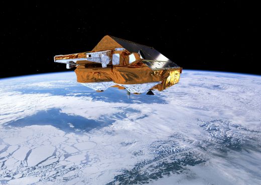
CryoSat-2 is the first successfully launched satellite in the CryoSat series. The mission, launched on 8 April, 2010, is operated by ESA as one of their Earth Explorer missions. It monitors changes in polar ice sheets.
Quick facts
Overview
| Mission type | EO |
| Agency | ESA |
| Mission status | Operational (extended) |
| Launch date | 08 Apr 2010 |
| Measurement domain | Land, Gravity and Magnetic Fields, Snow & Ice |
| Measurement category | Gravity, Magnetic and Geodynamic measurements, Landscape topography, Sea ice cover, edge and thickness, Ice sheet topography |
| Measurement detailed | Land surface topography, Sea-ice thickness, Sea-ice sheet topography, Gravity field |
| Instruments | Laser Reflectors (ESA), SIRAL, DGXX |
| Instrument type | Precision orbit, Radar altimeters |
| CEOS EO Handbook | See CryoSat-2 (Earth Explorer Opportunity Mission-2) summary |
Related Resources
Summary
Mission Capabilities
CryoSat-2 has three instruments onboard with the primary instrument being a radar altimeter named SIRAL (SAR (Synthetic Aperture Radar) Interferometer Radar Altimeter), which monitors land and sea ice sheet thickness to help explain the connection between the melting of polar ice and the rise in sea levels.
The other two instruments provide precise real-time orbit determination. A Doppler Orbitography and Radio-positioning Integrated by Satellite (DORIS) measures the frequency shift of radio signals transmitted by ground beacons to determine the orbital velocity of the satellite, while a Laser Retro-Reflector (LRR) receives pulses from laser tracking stations to determine orbital position.
Performance Specifications
SIRAL emits radio waves with a frequency of 13.575 GHz and a Pulse Repetition Frequency (PRF) dependent on the operating mode. Low-Resolution Mode (LRM) uses a PRF of 1.97 kHz, receives over a single channel, and is best when observing homogenous regions. SAR Mode (SARM) also receives over a single channel, however, uses a PRF of 17.8 kHz and is best used for observing sea ice. SAR Interferometric (SARIn) mode also uses a PRF of 17.8 kHz, however, receives over two channels, and is best at observing ice sheet boundaries. SIRAL has an along-track resolution of 250 m and a ground range resolution of 0.45 m. It is able to detect changes as small as 1.6 cm per year in the thickness of arctic sea ice, 3.3 cm per year in the thickness of land ice in small (103 - 104 km2) regions, and 0.17 cm per year in the thickness of land ice in large (106 km2) regions such as Antarctica.
CryoSat-2 undertakes a non-sun-synchronous orbit with an altitude of 717 km, an inclination of 92°, and experiences an orbital regression of 0.25° per day. The orbit has a period of 100 minutes and a repeat cycle of 369 days.
Space and Hardware Components
CryoSat-2 was launched in April 2010 from the Baikonur Cosmodrome in Kazakhstan aboard a Dnepr launch vehicle provided by the International Space Company Kosmotras. CryoSat-2 was built by Astrium with a weight of 720 kg. It received 85 modifications from the original CryoSat mission, which failed to launch in October 2005.
Telemetry, Tracking, and Command (TT&C) communications are performed via S-band radio frequencies with a 2 kbit/s uplink rate and an 8 kbit/s downlink rate. Payload data is transferred via X-band with a rate of 100 Mbit/s.
CryoSat-2 (Earth Explorer Opportunity Mission-2)
Spacecraft Launch Mission Status Sensor Complement Ground Segment References
Overview
CryoSat-2 is the follow-on Earth Explorer Opportunity Mission in ESA's Living Planet Program. It replaces CryoSat, which was selected for development in 1999 and lost as a result of launch failure on October 8, 2005.
CryoSat-2 will have the same mission objectives as the original CryoSat mission; it will monitor the thickness of land ice and sea ice and help explain the connection between the melting of the polar ice and the rise in sea levels and how this is contributing to climate change.
The original CryoSat mission was proposed by Duncan Wingham of the University College London (UCL) and an international science team. Duncan Wingham is also the mission PI. A nominal mission duration of three years is planned (excluding the commissioning and validation phases, which may last up to six months).
In Feb. 2006, ESA received the green light from its Member States to build and launch a CryoSat recovery mission, CryoSat-2, based on the same objectives as the original CryoSat mission. However, the design of the CryoSat-2 spacecrasft is being updated. The changes required to the design of CryoSat-2 were scrutinized from December 2006 to January 2007. The Δ-CDR (Critical Design Review) was completed on Feb. 1, 2007. 1) 2) 3) 4) 5)
A total of 85 improvements/modifications have been approved in the design of CryoSat 2 (of which 30-40% have been small software changes that make the satellite much easier to operate).
The new key features of CryoSat-2 include the following items:
• The SIRAL-2 (SAR/Interferometric Radar Altimeter-2) design includes a full backup SIRAL system, in case the primary payload malfunctions. Once in orbit, a special algorithm will be used to convert data collected by the CryoSat-2 satellite to create more accurate ice maps. - As a result of the dual SIRAL payload and associated interfaces, and other improvements to reliability, there has been a knock-on effect to the design of the satellite. For example, the backup SIRAL system has to be kept warm while it is switched off - the additional heater power is provided by increasing the size of the satellite's battery.
• A heat-radiating panel is being added. The path of CryoSat-2's orbit means it will face extremes of temperature. The panel ensures the electronics are protected
• Solar panels on the satellite's back are being added to account for the additional power requirements. Unlike many spacecrafts, CryoSat 2 does not have solar wings.
Preparatory Campaigns
In addition to building the new satellite, a number of field experiments to support the CryoSat-2 mission, were conducted or are getting underway in the Arctic. First is the Arctic Arc Expedition, part of the IPY (International Polar Year) 2007-2008. 6) 7)
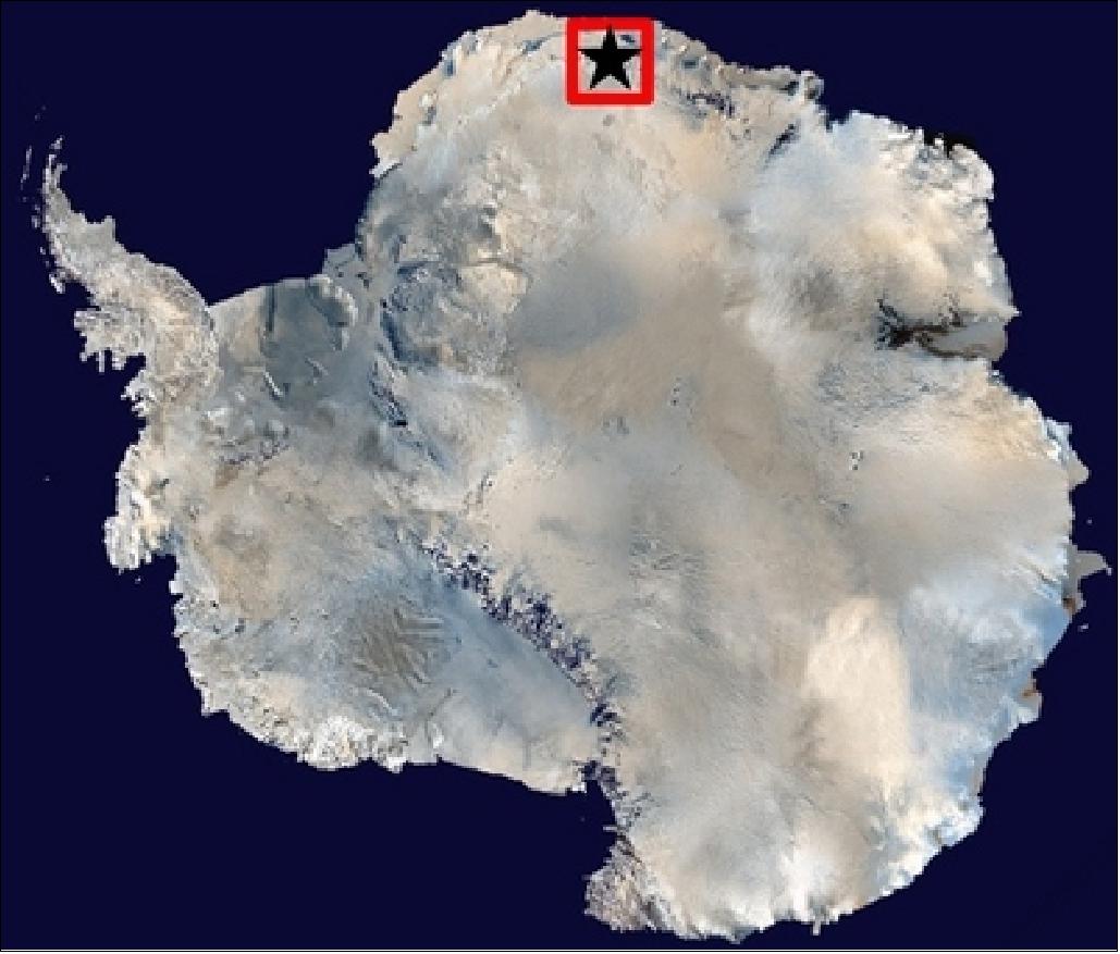
- Antarctic 2008/9 CroVEx campaign in the blue ice region (see Figure 1) in December 2008: German scientists from the Technical University of Dresden and the AWI (Alfred Wegener Institute) are spending up to four months venturing out onto the vast frozen reaches of what is known as the 'blue ice' region near the Russian Novo airbase in Dronning Maud Land in Antarctica. The aim is to take very accurate measurements of the surface topography, both from the air and on the ground to contribute to the validation program for CryoSat-2. 8)
In parallel to the efforts on the ground, the Alfred Wegner Institute (AWI) will be flying their POLAR5 aircraft across the blue ice site – starting just before Christmas and finishing before the New Year. From the plane, the AWI team will collect laser and radar height measurements along the very same tracks as the ground team. To do this they are using ESA's ASIRAS (Airborne Synthetic Aperture and Interferometric Radar Altimeter System), which simulates the measurements CryoSat.
- CryoVEx (CryoSat Validation Experiment) 2008 (3-week campaign in May 2008 in the far north of Greenland and Canada). CryoVEx 2008 is a continuation of a number of earlier campaigns that focus on collecting data on the properties snow and ice over land and sea. This year's campaign is a huge logistical undertaking as airborne, helicopter and ground measurements are being taken simultaneously in three different locations - out on the floating sea-ice north of the Canadian Forces Station Alert, on the Devon ice cap in Canada and on the vast Greenland ice cap.
A Twin Otter is carrying two key instruments: ASIRAS (Airborne SAR/Interferometric Radar System), a radar altimeter that mimics the radar altimeter onboard CryoSat-2, and a laser scanner which maps the surface beneath the plan, and a helicopter with an on-board sensor that measures sea-ice thickness. 9)
- In the spring of 2007, an international team of scientists stationed in Svalbard, Norway and two polar explorers are crossing the North Pole on foot. Both teams are part of a common effort to collect vital data on the ground and from the air in support of ESA's ice mission CryoSat-2.
The expedition's two Belgian explorers, Alain Hubert and Dixie Dansercoer, 'stepped' onto the sea ice off the coast of Siberia on March 1, 2007 each pulling a 130 kg sledge holding supplies and equipment. A parallel campaign by scientists from Germany, Norway and the UK is unfolding in the extreme northern archipelago of Svalbard, Norway. As part of the CryoVEx 2007 campaign (CryoSat-2 Validation Experiment), they are spending one month making measurements of snow and ice properties along long transects that crisscross the ice sheet surface.
- As the ground experiments are carried out, measurements are also being taken from the air by the Alfred Wegner Institute (AWI), Bremerhafen, Germany. The Dornier-228 aircraft carries the ASIRAS (Airborne SAR/Interferometric Altimeter System) instrument, which is an airborne version of the radar altimeter instrument onboard CryoSat-2. By comparing the airborne data with ground measurements scientists will test and verify novel methods for retrieving ice-thickness change from the CryoSat-2 satellite mission ahead of the launch.
- ASIRAS was built by Radar Systemtechnik (RST) of Switzerland with the support of the AWI and Optimare for the implementation and operation on an aircraft. It was test flown in March 2004 over the snow and ice expanses of Svalbard.
- The CryoVEx 2006 campaign took place April/May, 2006 and consisted of coordinated airborne and ground activities in support of CryoSat-2 validation goals over three land validation sites (Devon Island in Canada, Central Greenland and Svalbard, Spitzbergen, Norway) and a series of ice experiments over Alert / Ellesmere Island, Canada.
- LaRA (Laser and Radar Altimeter) campaign in the Arctic region of Greenland and Svalbard: The D2P (Delay-Doppler Phase-monopulse Radar) instrument of JHU/APL participated in this campaign which took place in May 2002 under joint NASA/ESA sponsorship to support calibration and validation activities, and science investigations in advance of the CryoSat and ICESat missions. The D2P radar altimeter was flown aboard the NASA-P3 aircraft along with the ATM (Airborne Topographic Mapper) laser altimeters to collect simultaneous laser and radar altimeter (hence, the LaRA campaign) measurements over land and sea ice.
- CryoVEx (CryoSat Validation Experiment) campaign: As a follow-on to the LaRA campaign, the D2P system was flown again in 2003 under joint NASA/ESA sponsorship as part of the CryoVEx field campaign. As in 2002, simultaneous laser and radar altimeter measurements were collected in the Arctic.
Such painstaking ground work is necessary to be able of measuring ice thickness down to centimeter level (1-3 cm average) from space. This in turn may lead to a better understanding of the impact that changing climate is having on the polar ice fields. See also the D2P and ASIRAS descriptions on the eoPortal (along with the campaigns for the validation of the SIRAL instrument).
Many more CryoVEx campaigns were conducted throughout the CryoSat-2 mission (up to 2018) as provided in the ASIRAS file on the eoPortal.
Spacecraft
The CryoSat-2 spacecraft is being built and integrated by EADS Astrium GmbH of Friedrichshafen, Germany, as prime contractor of a consortium.
- The spacecraft structure consists of a long rectangular main platform body, surmounted by fixed solar arrays in the form of a tent.
- The spacecraft has neither deployable appendages nor any other moving parts except for thruster valves.
- The lower surface of this structure is permanently earth facing.
- All electronics are mounted on the nadir plate acting as radiator.
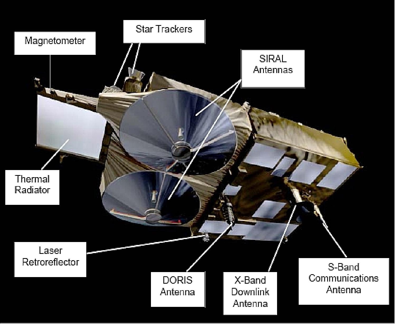
- The antennas used for radio communication, and the Laser Retroreflector, are mounted on this surface; an emergency antenna for command and monitoring is also fitted on top of the satellite between the solar arrays.
- The two SIRAL instrument antenna dishes are mounted on a separate rigid bench in the forward section of the S/C.
- In addition, a dedicated SIRAL radiator is mounted at the nose tip. 10)
The spacecraft is 3-axis stabilized. A slight nose-down attitude of the S/C (6º) is chosen (using magnetorquers and 10 mN cold-gas thrusters) to ensure minimum attitude correction due to gravity-gradient disturbances. The S/C has dimensions of 4.6 m x 2.34 m x 2.20 m. The S/C mass is about 720 kg (including 36 kg propellant), the design life is 3.5 years (goal of 5.5 years). Spacecraft power generation is provided by two triple-junction GaAs solar arrays with an efficiency of 27.5% (two oriented solar panels), each panel provides power of 850 W at normal solar incidence. A PCDU (Power Control and Distribution Unit) provides onboard distribution. The energy is stored by a lithium-ion battery (60 Ah capacity).
The pointing requirements are the main design drivers for the AOCS: 11)
• High precision cross-track pointing knowledge of < 10 arcsec for SARIn mode (SARIn refers to the SAR interferometric mode).
• S/C attitude maintenance with a pointing accuracy of < 0.2º per axis and a pointing stability of < 0.005º for 0.5 s in the nominal Earth-pointing phase of the mission
• Provision of very low disturbances due to thruster activity to meet the very high precise orbit determination (POD) accuracy of the CryoSat orbit.
• The AOCS (Attitude Orbit and Control Subsystem) comprises the following elements:
- A cold gas system (RCS) for attitude control and orbit transfer and maintenance maneuvers, 16 attitude control thrusters (10 mN) and 4 orbit control thrusters (40 mN). Nitrogen is used as propellant (132 l tank). 12)
- A set of 3 magnetorquers is used for compensation of environmental disturbance torques in support of RCS. The MT30-2-GRC, originally developed and qualified for the GRACE mission by ZARM Technik GmbH, has been selected for CryoSat.
- A set of three star tracker heads (also a part of the payload) providing autonomous inertial attitude determination for the spacecraft. The multiple configuration makes the sensor system one-failure tolerant, except for the rare occurrence of simultaneous sun and moon blinding of two heads, to which the system software is tolerant.
Consequently, two camera heads are operated in parallel at all times to cope with sun-blinding. In its acquisition mode, which takes 2-3 seconds, the star tracker calculates a coarse attitude by matching triangle patterns of stars with patterns stored in its catalog. Subsequently, in attitude update mode it calculates precise attitude at a rate of 1.7 Hz.
The star tracker attitude serves also as reference for determining the orientation of the SIRAL interferometric baseline. The orientation of the interferometric baseline needs to be very accurately measured in-flight: small errors in knowledge of the roll-angle translate into substantial errors in the elevation of off-nadir points.
The HE-5AS star tracker of Terma A/S, originally developed and qualified for the NEMO (Navy EarthMap Observer) and FCT (Foreign Comparative Test) projects, is selected for CryoSat. It is a fully autonomous star tracker capable of delivering high-accuracy inertial attitude measurements from a lost-in-space condition with no external attitude information. The EOL performance of the star tracker is < 3.2 arcsec in the lateral axes and < 16 arcsec about the roll axis under worst-case conditions. 13)
The star tracker baffle has been designed to meet the required sun exclusion angle of 30º and the moon exclusion angle of 25º. These exclusion angles ensure together with the star tracker accommodation on the antenna bench that during the whole mission sun and moon can only blind one star tracker head at any time.
• A DORIS receiver is part of an overall system, for real-time measurements of satellite position, velocity and time. DORIS measures the Doppler frequency shifts of UHF and S-band signals transmitted by ground beacons. Its measurement accuracy is < 0.5 mm/s in radial velocity allowing an absolute determination of the orbit position with an accuracy of 2-6 cm (see DORIS and LLR description under sensor complement). -
The DORIS system comprises a network of more than 50 ground beacons, a number of receivers on several satellites in orbit and in development, and ground segment facilities. It is part of the International DORIS Service, the IDS, which also offers the possibility of precise localization of user beacons.
• CESS (Coarse Earth-Sun Sensor) of CHAMP and GRACE heritage (a patented design of Astrium GmbH). Provides attitude measurements (<5º) with respect to the sun and Earth for initial acquisition and coarse pointing. The FOV of CESS is a full spherical one, i.e. no special search maneuvers are necessary to find the Earth or the sun. Its measurement principle is based The concept is based on temperature differences measured by 6 omnidirectional arranged sensor heads (PT1000 thermistors).
• A set of three three-axis fluxgate magnetometers are used for magnetorquer control and as rate sensors. They provide a measurement range of at least ± 60.000 nT with an accuracy of better than 0.5 % full scale.
The AOCS provides high pointing accuracy (a few tens of an arcsecond), knowledge and stability in nominal Earth-pointing. It also has to perform the orbit changes between the science and validation phase orbits. The AOCS uses inertial attitude measurements from the set of 3 star tracker camera head units and DORIS real-time navigation to convert the inertial attitude into Earth referenced attitude (star sensor FOV of 22º x 22º, ).
- The RCS (Reaction Control Subsystem), developed at PolyFlex Space Ltd. (a Marotta UK Ltd. company), is a cold gas propulsion system for auxiliary attitude control (in which it provides deadband protection around the axis defined by the instantaneous geomagnetic field) and for orbit transfer and maintenance maneuvers. It has 16 attitude control thrusters of 10 mN each and 4 orbit control thrusters of nominally 40 mN each. A single high-pressure tank stores 36.2 kg of nitrogen gas at 278.6 bar. 14) 15)
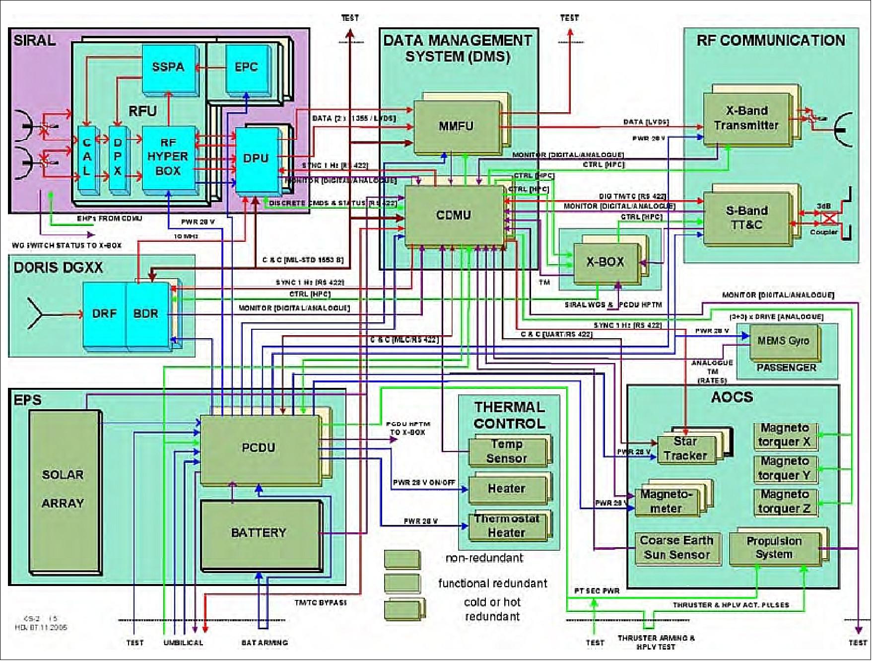
The CDMU (Control and Data Management Unit), consisting of a processor and a hardware-based fault detection system, handles all on-board command and control functions including telecommand decoding and the AOCS processing functions (the OBC is based on the ERC-32 microprocessor). A MIL-STD-1553B communications bus is used as payload interface (for SIRAL and DORIS). The on-board solid-state memory has a capacity of 2 x 128 Gbit.
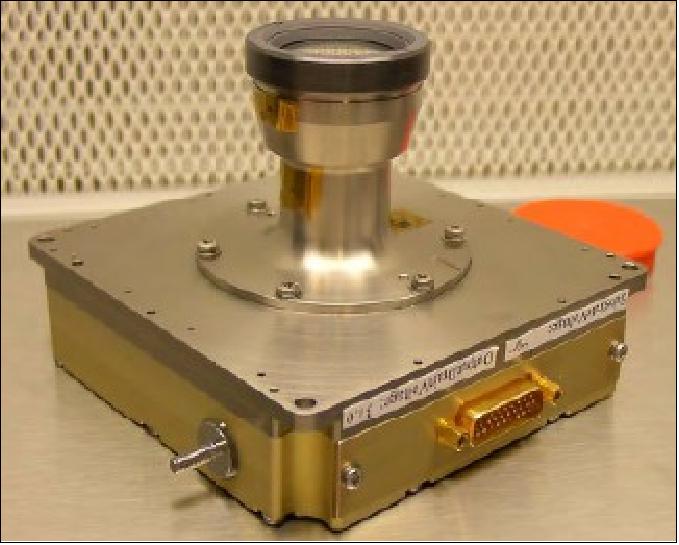
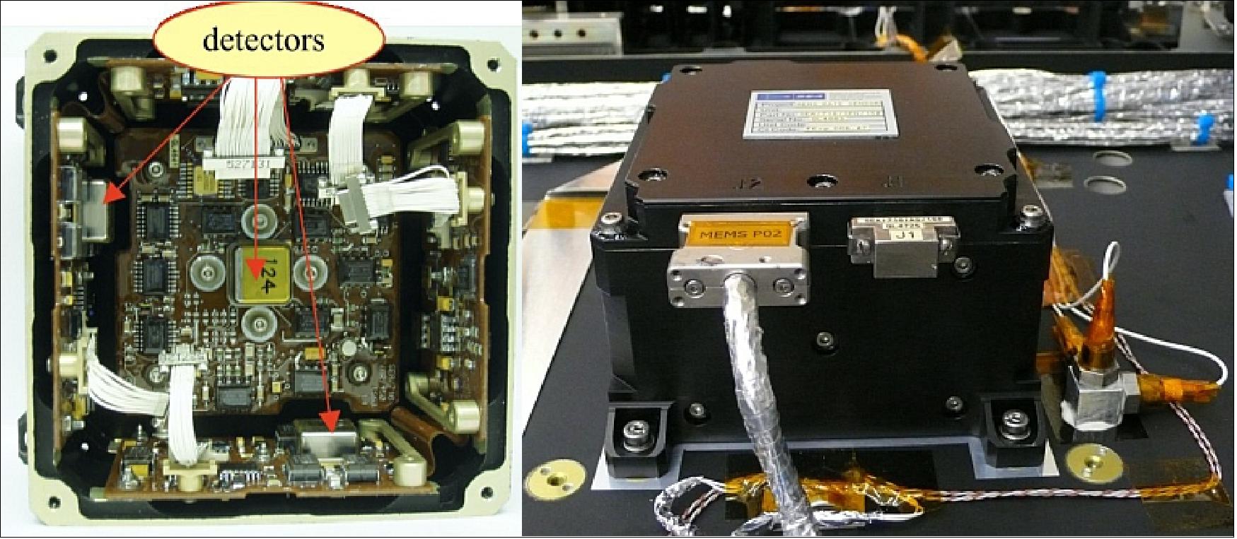
• Experimental Rate Sensor: CryoSat-2 carries a small technology experiment as a passenger. This device is an attitude rate sensor based on MEMS (Micro-Electro-Mechanical-Systems) technology in which microelectronics and mechanical devices (in this case a sensor) are fabricated on the same substrate. The MEMS sensor detects attitude rate to provide the same function as a more traditional gyro and is based on a device widely used in in-car navigation systems. Three orthogonal MEMS sensors are mounted in the experiment, to measure 3-axis attitude rates. The unit is called MRS (MEMS Rate Sensor) in the CryoSat context. The goal is to provide a low-cost rate-sensor or gyro. The device is provided free of charge to CryoSat-2 in exchange for the flight opportunity (Ref. 10).
The measurement data are not used on-board and only sent in housekeeping telemetry to the flight control centre. Here they will be used as an additional data type in monitoring satellite dynamics during attitude transitions.
In the context of the technology program in which the MRS has been developed, it is called SiREUS-FExp, for European Silicon Rate Sensor Flight Experiment. - SiREUS is a compact and lightweight solid-state MEMS rate sensor which was developed in the context of an ESA technology technology program. The UK development team consisted of the following partner organizations: AIS (Atlantic Inertial Systems - formerly BAE Systems of Plymouth), SEA (Systems Engineering & Assessment Ltd. of Bristol), and SELEX-GALILEO a Finemeccanica owned company (formerly BAE Systems of Edinburgh). This development is based on the established BAE SYSTEMS automotive MEMS detector, however significant developments were required to meet the performance requirements while achieving compatibility of the electronics to the space environment and ensuring low recurring price. The partnership with a significant commercial provider such as AIS should be emphasized as a critical aspect of the program. 16) 17) 18)
Parameter | Requirement | MRS status |
Configuration | 3-axis, rate or integration mode (an optimized mechanical and electronics configuration) | OK |
Instrument mass | < 0.75 kg (electronics and mechanical architecture commensurate with MEMS detector) | 0.745 kg |
Power consumption (nominal) | < 3.5 W | 5.4 W |
Bias stability (3σ), ΔΤ < ±10ºC | 5 to 10º/h over 24 hours (this represents a factor 10 improvement on best existing MEMS devices) | 10-20º/h |
Angular random walk | < 0.2º/h1/2 | 0.04º/h1/2 |
Range | Up to 20º/s | OK |
Interface | RS-422, SpaceWire, analog | RS-422, analog |
Mission | 18 years in GEO (this required radiation hardened implementation and ITAR free electronics) | OK |
The SiREUS unit has met or exceeded the key performance requirements set at the start of the program. The unit does not contain any software; all control loops are implemented digitally in an FPGA. The SiREUS unit is fairly compact, but its size is currently dominated by analog electronics, not the MEMS. It may be cost effective to achieve a significant reduction in mass and volume, if this results in a match with many more customer requirements.
SiREUS has demonstrated that it is possible to construct multi-lateral programs to spin-in technology from non space industry organizations and to make significant improvements in the performance of the 'spin-in' technology. There are positive signs for the wider application of this technology in 'spin-off' programs. The instrument has a size of 100 mm x 100 mm x 70 mm.
Spacecraft dimensions | 4.60 m x 2.34 m x 2.20 m |
Spacecraft mass | 720 kg (inclusive 37 kg of fuel) |
Spacecraft power | 2x GaAs body-mounted solar arrays, with 850 W each at normal solar incidence; 78 Ah Li-ion battery |
Attitude | 3-axis stabilized local-normal pointing, with 6º nose-down attitude, using magneto-torquers and 10 mN cold-gas thrusters |
Data volume | 320 Gbit/day |
On-board data storage | 256 Gbit use of SSR (Solid State Recorder) |
Spacecraft design life | 3.5 years (goal of 5.5 years) |
Launch
The CryoSat-2 spacecraft was launched on April 8, 2010 on a Dnepr vehicle from the Baikonur Cosmodrome, Kazakhstan. The launch provider was ISC (International Space Company) Kosmotras. 19) 20) 21)
Note: The technical issue with the second stage of the Dnepr rocket that delayed the launch of ESA's Earth Explorer CryoSat-2 satellite in February 2010 has now been resolved – and the new launch date of 8 April has been set. The fuel reserve problem of the second stage surfaced a week before the scheduled launch date and after the 'space head module', encasing the CryoSat-2 satellite, had been mated to the rest of the rocket in the launch silo. Consequently, the space head was returned to the integration facilities pending an investigation and new launch date. 22)
The delay, from the planned launch date of Dec. 2009, is due to the limited availability of facilities at the Baikonur launch site in Kazakhstan, which is particularly busy at the moment. 23)
Orbit
Non sun-synchronous circular LEO orbit, mean altitude = 717 km, inclination = 92º, nodal regression of 0.25º per day. Ground track repeat cycle: 369 days (with 30 day pseudo subcycles). This configuration allows a sufficient coverage for the polar regions.
The CryoSat mission requirements include:
• An orbit change is required during the mission with the objective to visit at least twice a validation orbit, approximately 6 km lower in altitude than the science phase orbit
• The payload must be operated in various modes, as a function of geographical region, such that the orbital operations, and data sets collected, on successive orbits are dissimilar
• The payload utilization demands very precise orbit and attitude restitution. Minimum operations of three years are required.
The CryoSat mission is aimed in part at gaining coincident coverage with the GLAS laser altimeter of the NASA ICESat mission.
The following support phases are defined:
• Commissioning phase: The nominal duration is two months. During this phase the satellite and its payload are brought into a fully operating condition in its nominal orbit.
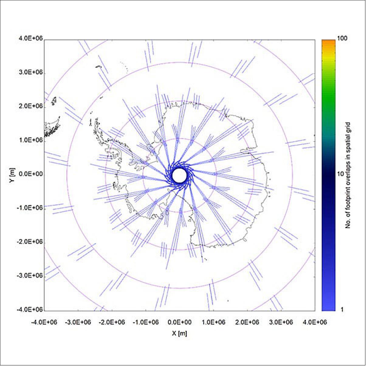
• Science phase: This includes a long-repeat cycle [a 369-day orbit (5344 revolutions) repeat phase will be used, with a 30-day subcycle]. The science phase is the nominal operational support mode of the mission. This orbit is designed to provide very dense orbit cross-overs above 72º of latitude, for use over the ice sheets. With coverage to 88º of latitude, all but a very small area of the land and marine ice fields will be within the coverage of the satellite. In addition, the 30 day subcycle provides approximately monthly coverage of the sea ice fluctuations.
• Validation phases: The objective is to conduct calibration or validation experiments that are at a fixed locations on Earth. In these phases the satellite may be placed into a 2-day repeat orbit. A validation phase may have a duration of up to 1 month, and there may be more than one during the mission lifetime. The measurements made by the satellite mission will need to be verified by ground-based experiments.
RF communications: The S-band link is used for all TT&C communications (2 kbit/s uplink and 8 kbit/s downlink). The physical downlink operates at 16 kbit/s but carries an overhead of error correction coding. The X-band downlink (center frequency of 8.100 GHz) provides a payload transfer rate of 100 Mbit/s. All onboard data are stored in the MMFU (Mass Memory and Formatting Unit) of 2 x 128 Gbit (EOL) capacity. Data arrive at the MMFU directly from the SIRAL instrument on a pair of fast IEEE 1355 standard serial links (SpaceWire for the two high-rate interferometric data channels) and via the MIL-STD-1553 bus for the low rate data channels. Data are also transferred from the CDMU and the DORIS over the MIL-STD-1553 bus. About 320 Gbit/day of onboard source data are being generated and transmitted to the ground.
Mission Status
• August 23, 2023: A new CryoSat sea level anomaly product designed to enable ocean science and the development of operational marine applications has been released.
The dataset, presented in the Nature Research journal Scientific Data, provides a unique perspective on ocean surface levels, thanks to the mission’s novel orbit and its extended lifespan of more than 13 years.
It was produced and verified by the UK’s National Oceanography Centre (NOC) as part of a wider ESA-backed project to validate CryoSat ocean products. The products are available for download here.
• July 12, 2022: The CryoSat-2 satellite is currently being aligned with ICESat-2 over Antarctica, unlocking fresh possibilities in the wealth of new information being delivered by the near-synchronous orbit of the two satellites. 24)
- Between 16 and 31 July 2020, a campaign dubbed CRYO2ICE took off, where ESA raised the orbit of its Earth Explorer CryoSat-2, to periodically align with NASA's ICESat-2 satellite.
- The campaign's aim was to achieve a partial parallel ground-track every 19th revolution of CryoSat-2 and every 20th revolution of ICESat-2—allowing data in the polar areas to be collected by the two satellites within a few hours of each other.
- To reach this goal, CryoSat-2's semi-major axis had to be increased by 887 metres through a series of 14 manoeuvres.
- The scientific benefits that such a small orbit change for CryoSat-2 brought were impressive. By using the combined data from CryoSat-2's radar and ICESat-2's laser instruments, inaccuracies in sea ice thickness and land ice measurements were reduced for the first time. In addition, it enabled to map snow at the poles and improve climate models, among other aspects.
- On top of that, the quality of coincidences is increasing as time goes by because the orbital planes of CryoSat-2 and ICESat-2 are gently coming closer to each other. This is the result of the natural perturbations affecting the orbits, and there is a direct link between the orbital plane separation and time difference between ICESat-2/CryoSat-2 observations, when we have a coincident track. This natural evolution in the satellites' orbit offers a benefit to scientists in obtaining the combined data.
- In July this year (2022), the orbital plane separation will reach 25 degrees, and decreasing. This translates into a time difference of approximately 1 hour and 40 minutes between observations at that time (it was three hours when the campaign first started), decreasing at a rate of approximately 40 minutes per year. This means that, in about 2.5 years, we will have quasi-synchronous, co-spatial coincidences.
- The orbit in which CryoSat-2 is currently flying has a 19/20 revolution resonance with ICESat-2. This enables recurring coincidences with the ICESat-2 instrument every 1.33 days. That is, every 1.33 days there is a coincident track (spatial). A coincidence, however, cannot be maintained for a very long fraction of the orbital period; after a while the ground tracks start diverging from each other.
- This is why experts keep them at the areas of interest for these two missions: the poles. The parameter to control this is the orbital phase. Since CryoSat-2 acquired the resonant orbit with ICESat-2 in 2020, it has been flying at an orbital phase such that the coincidences occur in the areas close to the North Pole.
- The purpose of the current campaign is to change the orbital phase of the CryoSat-2 satellites, in order to maximise coincidences in the Antarctic region (at the expense of reducing them at the North Pole).
- This idea concerns the geographic (spatial) collocation between observations taken by each of the spacecraft. But the observations are not taken simultaneously. In fact, what happens for those coincident tracks is that ICESat-2 first passes over a certain area, and then CryoSat-2 follows over the same location some time later. This time difference is a very important parameter for the quality of a coincidence: ice—which constantly moves—is being observed, and the conditions change. Therefore, the lower the time difference, the better.
- Overall, this translates into huge results for scientists characterising snow loads, improving the retrieval of sea ice thickness, and ultimately, the understanding of the ongoing changes in the cryosphere due to climate change.
- Javier Sanchez, Flight Dynamics Engineer at ESA, states, "The satellites operate at completely different altitudes. But with the satellites in this configuration we have a mechanism put in place in space, which delivers recurring coincidences between their instruments every 1.3 days. And this is done in a passive manner, meaning that each one of the satellites is able to continue with their own mission autonomously."
- Tommaso Parrinello, ESA's CryoSat Mission Manager, concludes, "Since we started CRYO2ICE, the scientific community have been very excited about this programme. It is delivering a unique and probably unrepeatable data record, which will help us to improve our understanding on how the cryosphere is responding to global warming and, at the same time, improve also the past climate records, especially now over Antarctica."
• November 3, 2021: As world leaders and decision-makers join forces at COP26 to accelerate action towards the goals of the Paris Agreement, new research, again, highlights the value of satellite data in understanding and monitoring climate change. This particular new research, which is based on measurements from ESA's CryoSat-2 mission, shows that extreme ice melting events in Greenland have become more frequent and more intense over the past 40 years, raising sea levels and the risk of flooding worldwide. 25)
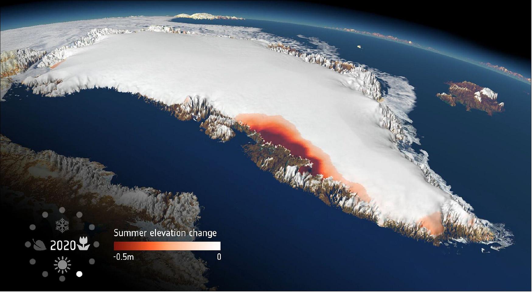
- The findings, published this week in Nature Communications, reveal that Greenland's meltwater runoff has risen by 21% over the past four decades, and has become 60% more erratic from one summer to the next. 26)
- Over the past decade alone, 3.5 trillion tons (3.5 x 10¹² tons) of ice have melted from the Greenland ice sheet and spilled into the ocean. This is enough to cover the entire UK with meltwater 15 meters deep or cover the entire city of New York with meltwater 4500 meters deep.
- The research was funded by ESA as part of its Polar+ Surface Mass Balance Feasibility project and used measurements from the Agency's ice mission CryoSat-2 — and it is the first study to use satellite data to detect ice-sheet runoff from space.
- Lead author, Dr Thomas Slater, a research fellow in the Centre for Polar Observation and Modelling at the University of Leeds in the UK said, "As we've seen with other parts of the world, Greenland is also vulnerable to an increase in extreme weather events."
- "As our climate warms, it's reasonable to expect that the instances of extreme melting in Greenland will happen more often – observations such as these are an important step in helping us to improve climate models and better predict what will happen this century."
- The research shows that between 2011 and 2020 meltwater runoff from Greenland raised the global sea level by 1 cm. Worryingly, one third of this total was produced in just two separate years, in 2012 and 2019 – two hot summers when extreme weather led to record-breaking levels of ice melting not seen in the past 40 years.
- Raised sea levels caused by ice melt heightens the risk of flooding for coastal communities worldwide and disrupts Arctic Ocean marine ecosystems on which indigenous communities rely for food. It can also alter patterns of ocean and atmospheric circulation, which affect weather conditions around the planet.
- During the past decade, runoff from Greenland has averaged 357 billion tons per year, reaching a maximum of 527 billion tons of ice melt in 2012, when changes in atmospheric patterns caused unusually warm air to sit over much the ice sheet. This was more than twice the minimum runoff of 247 billion tons that occurred in 2017.
- The changes are related to extreme weather events, such as heatwaves, which have become more frequent and are now a major cause of ice loss from Greenland because of the runoff they produce.
- Dr Slater said, "There are, however, reasons to be optimistic. We know that setting and meeting meaningful targets to cut emissions could reduce ice losses from Greenland by a factor of three, and there is still time to achieve this."
- These first observations of Greenland runoff from space can also be used to verify how climate models simulate ice sheet melting which, in turn, will allow improved predictions of how much Greenland will raise the global sea level in the future as extreme weather events become more common.
- Study co-author, Dr Amber Leeson, Senior Lecturer in Environmental Data Science at Lancaster University in the UK, said, "Model estimates suggest that the Greenland ice sheet will contribute between about three and 23 cm to global sea-level rise by 2100.
- "This prediction has a wide range, in part because of uncertainties associated with simulating complex ice-melt processes, including those associated with extreme weather. These new spaceborne estimates of runoff will help us to understand these complex ice-melt processes better, improve our ability to model them, and thus enable us to refine our estimates of future sea-level rise."
- Finally, the study shows that polar-orbiting satellite altimeters are able to provide instant estimates of summer ice melting, which supports efforts to expand Greenland's hydropower capacity, and Europe's ambition to launch the Copernicus Sentinel Expansion CRISTAL mission to eventually succeed CryoSat-2.
- ESA's CryoSat-2 mission manager, Dr Tommaso Parrinello, said, "Since it was launched over 11 years ago, CryoSat-2 has yielded a wealth of information about our rapidly changing polar regions.
- "This remarkable satellite remains key to scientific research and the indisputable facts, such as these findings on meltwater runoff, that are so critical to decision-making on the health of our planet.
- "Looking further to the future, the Copernicus Sentinel Expansion mission CRISTAL will ensure that Earth's vulnerable ice will be monitored in the coming decades. In the meantime, it is imperative that CryoSat remains in orbit for as long as possible to reduce the gap before these new Copernicus missions are operational."
• June 10, 2021: Research based on ice-thickness data from ESA's CryoSat-2 and Envisat missions along with a new model of snow has revealed that sea ice in the coastal regions of the Arctic may be thinning twice as fast as thought. 27)
- Frequently in the news, Earth's declining ice is without doubt one of the biggest casualties of climate change. However, calculating the amount of ice we are losing can be a challenge.
- While monitoring the area of land and ocean covered by ice is relatively straightforward using images from satellites carrying camera-like instruments, scientists need to understand how the actual volume is changing – and to calculate this, they need measurements of ice thickness.
- ESA's CryoSat altimeter returns readings of ice height by timing how long it takes for radar waves to bounce back to the satellite from the ice surface. When it comes to ice floating in the polar oceans, ice thickness is inferred by measuring the height of the ice above the water.
- However, these measurements can be distorted by the weight of overlying snow pushing it down into the ocean water. Scientists adjust for this effect using a map of average snow depth based on historical field measurements, but this map is now out of date and does not account for the impact of climate change on Arctic snowfall and regional snow-depth variations.
- A paper, published recently in The Cryosphere, describes how researchers swapped the old map of snow depth for the results of a new computer model that calculates snow depth and density using inputs such as air temperature, snowfall and ice motion to track how much snow accumulates on sea ice as it moves around the Arctic Ocean. 28)
- By combining the results of the snow model with radar observations from CryoSat and Envisat, they estimated the overall rate of decline of sea-ice thickness in the Arctic, as well as the variability of sea-ice thickness from year to year.
- They concluded that sea ice in key Arctic coastal regions is thinning at a rate of 70–100% faster than previously thought. In particular, they found that in the coastal regions of Laptev, Kara and Chukchi seas, the rate at which ice is thinning increased by 70%, 98% and 110% respectively, when compared to earlier calculations.
- Robbie Mallett, PhD student at the Centre for Polar Observation and Modelling (CPOM) at UCL in the UK, said, "The thickness of sea ice is a sensitive indicator of the health of the Arctic. It is important as thicker ice acts as an insulating blanket, stopping the ocean from warming up the atmosphere in winter, and protecting the ocean from the sunshine in summer. Thinner ice is also less likely to survive during the Arctic summer melt."
- "Previous calculations of sea-ice thickness are based on a snow map that was last updated 20 years ago. Because sea ice has begun forming later and later in the year, the snow on top has less time to accumulate. Our calculations account for this declining snow depth for the first time, and suggest the sea ice is thinning faster than we thought."
- Prof. Julienne Stroeve at CPOM added, "There are a number of uncertainties in measuring sea-ice thickness, but we believe our new calculations are a major step forward in terms of more accurately interpreting the data we have from satellites."
- "We hope this work can be used to better assess the performance of climate models that forecast the effects of long-term climate change in the Arctic – a region that is warming at three times the global rate, and whose millions of square kilometers of ice are essential for keeping the planet cool."
- Michel Tsamados, also a researcher at CPOM, explained, "As part of the ESA Polar Science Cluster, we are actively developing complementary methods based on multi-frequency multi-satellite data fusion to further increase our understanding of the snow on sea-ice cover and its role in the climate and remote sensing of the polar regions."
- As well as the consequences for feedback mechanisms in the way Earth's climate works, thinning sea ice in the coastal Arctic seas has implications for human activity in the region, both in terms of shipping along the Northern Sea Route, as well as the extraction of resources from the sea floor such as oil, gas and minerals. It is also a concern for indigenous communities as it leaves settlements on the coast increasingly exposed to wave action from the emerging ocean.
- This study further confirms the key importance of enhancing our capability of simultaneously monitoring snow depth and sea-ice thickness change over the Arctic which is a primary objective of CRISTAL, one of future Copernicus expansion missions.
- The UK's Natural Environment Research Council, ESA's Earth Observation Science for Society program and NASA funded this research.
• June 01, 2021: As our climate warms, ice melting from glaciers around the world is one of main causes of sea-level rise. As well as being a major contributor to this worrying trend, the loss of glacier ice also poses a direct threat to hundreds of millions of people relying on glacier runoff for drinking water and irrigation. With monitoring mountain glaciers clearly important for these reasons and more, new research, based on information from ESA's CryoSat mission, shows how much ice has been lost from mountain glaciers in the Gulf Alaska and in High Mountain Asia since 2010. 29)
- Monitoring glaciers globally is a challenge because of their sheer number, size, remoteness and rugged terrain they occupy. Various satellite instruments offer key data to monitor change, but one type of spaceborne sensor – the radar altimeter – has seen limited use over mountain glaciers.
- Traditionally, satellite radar altimeters are used to monitor changes in the height of the sea surface and changes in the height of the huge ice sheets that cover Antarctica and Greenland. They work by measuring the time it takes for a radar pulse transmitted from the satellite to reflect from Earth's surface and return to the satellite. Knowing the exact position of the satellite in space, this measure of time is used to calculate the height of the surface below.
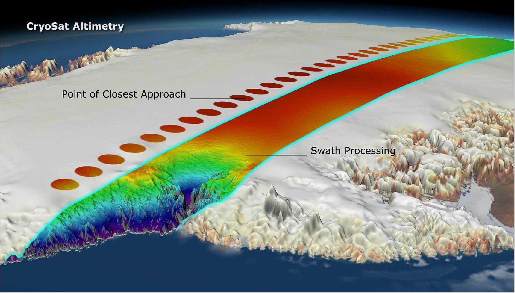
- However, the footprint of this type of instrument is generally too coarse to monitor mountain glaciers. ESA's CryoSat pushes the boundaries of radar altimetry and a particular way of processing its data – swath processing – make it possible to map glaciers in fine detail.
Figure 14: As our climate warms, ice melting from glaciers around the world is one of main causes of sea-level rise. As well as being a major contributor to this worrying trend, the loss of glacier ice also poses a direct threat to hundreds of millions of people relying on glacier runoff for drinking water and irrigation. Using information from ESA's CryoSat mission, new research shows that between 2010 and 2019, the Gulf of Alaska lost 76 Gt of ice per year while High Mountain Asia lost 28 Gt of ice per year. These losses are equivalent to adding 0.21 mm and 0.05 mm to sea level rise per year, respectively (video credit: Planetary Visions/ESA)
- A paper published recently in The Cryosphere describes how scientists used CryoSat to investigate ice loss in the Gulf of Alaska and High Mountain Asia. 30)
- They found that between 2010 and 2019, the Gulf of Alaska lost 76 Gt of ice per year while High Mountain Asia lost 28 Gt of ice per year. These losses are equivalent to adding 0.21 mm and 0.05 mm to sea level rise per year, respectively. Note: 1Gt corresponds to a volume of 1 km3.
- Livia Jakob, from Earthwave, explains, "One of the unique properties of this dataset is that we can look at ice trends at exceptionally high resolution in space and time. This enabled us to discover changes in trends, such as the increased ice loss from 2013 onwards in parts of the Gulf of Alaska, which is linked to climatic changes."
- The study, which was carried out through ESA's Science for Society program, also shows that almost all regions have lost ice, with the exception of the Karakoram-Kunlun area in High Mountain Asia, a phenomenon known was the ‘Karakoram anomaly'.
- Noel Gourmelen, from the University of Edinburgh, said, "It is astonishing to think that over last decade alone, both regions have lost 5% of their volume of ice. What CryoSat has accomplished also is astonishing. While glaciers were a secondary objective of the mission, few would have thought possible to use radar altimetry in regions with extremely complex topography like High Mountain Asia and the Gulf of Alaska.
- "But thanks to a brilliant altimeter design, dedicated support from ESA, and many years of research by the community, interferometric radar altimeters are now part of the toolset to monitor glacier change globally."
- This research, as well as that published in a related paper covering the entire Arctic region apart from Greenland, demonstrates that this unique high-resolution radar altimetry dataset can provide crucial information to better quantify and understand glacier changes on a global scale. This also opens up possibilities to monitor glaciers globally with satellites such as the planned CRISTAL mission, part of the expansion of Europe's Copernicus program.
• May 21, 2021: With alarm bells ringing about the rapid demise of sea ice in the Arctic Ocean, satellite data have revealed how the intrusion of warmer Atlantic waters is reducing ice regrowth in the winter. In addition, with seasonal ice more unpredictable than ever, ESA's SMOS and CryoSat-2 satellites are being used to improve sea-ice forecasts, which are critical for shipping, fisheries and indigenous communities, for example. 31)
- The amount of sea ice floating in the Arctic Ocean varies enormously as it grows and shrinks with the seasons. Although some of the older thicker ice remains throughout, there is an undeniable trend of declining ice as climate change tightens its grip on this fragile polar region.
- Arctic sea ice reaches a maximum around March after the cold winter months and then shrinks to a minimum around September after the summer melt. However, these seasonal swings are not only linked to the changing seasons – it transpires that along with our warming climate, the temperature of adjacent ocean seawater is now also adding to the ice's vulnerability.
- Previous research suggested that sea ice is able to recover in the winter following a strong summer melt because thin ice grows faster than thick ice. However, new findings that heat from the Atlantic Ocean is overpowering this stabilizing effect – reducing the volume of sea ice that can regrow in the winter. This means that sea ice is more vulnerable during warmer summers and winter storms.
- Robert Ricker, from the AWI Helmholtz Centre for Polar and Marine Research in Germany, and colleagues mapped regional changes in sea-ice volume owing to drift and calculated how much ice grows because of freezing each month. They also used model simulations to explore the causes of change, which corroborated their findings.
- Dr Ricker said, "Over the last decades we observed the tendency that the less ice you have at the beginning of the freezing season, the more it grows in the winter season.
- "However, what we've found now is that in the Barents Sea and Kara Sea regions, this stabilizing effect is being overpowered by ocean heat and warmer temperatures that are reducing the ice growth in winter."
- This new process is called Atlantification, meaning that heat from the Atlantic Ocean carried to higher latitudes is causing the edge of the sea ice to retreat.
- "Importantly, this also means that if you have a warm summer or strong winds, the sea ice is less resilient," added Dr Ricker.
- The researchers believe that the stabilizing mechanism in other regions of the Arctic could also be overpowered in the future.
- While it is clearly essential to continue monitoring Arctic sea ice for evidence to support climate policies, satellite observations are put to practical use such as sea-ice forecasting.
- Ice-thickness data from the CryoSat mission played an important contribution to the Atlantification findings, but the mission's data combined with data from the SMOS satellite are also key to improving forecasts of the thinner more fragile thin sea ice.
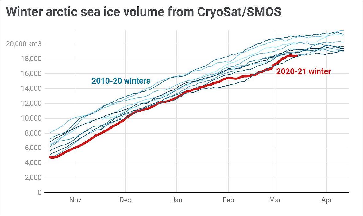
- The Alfred Wegner Institute (AWI) in Germany merge weekly CryoSat data with daily SMOS data to generate a weekly-averaged product every day.
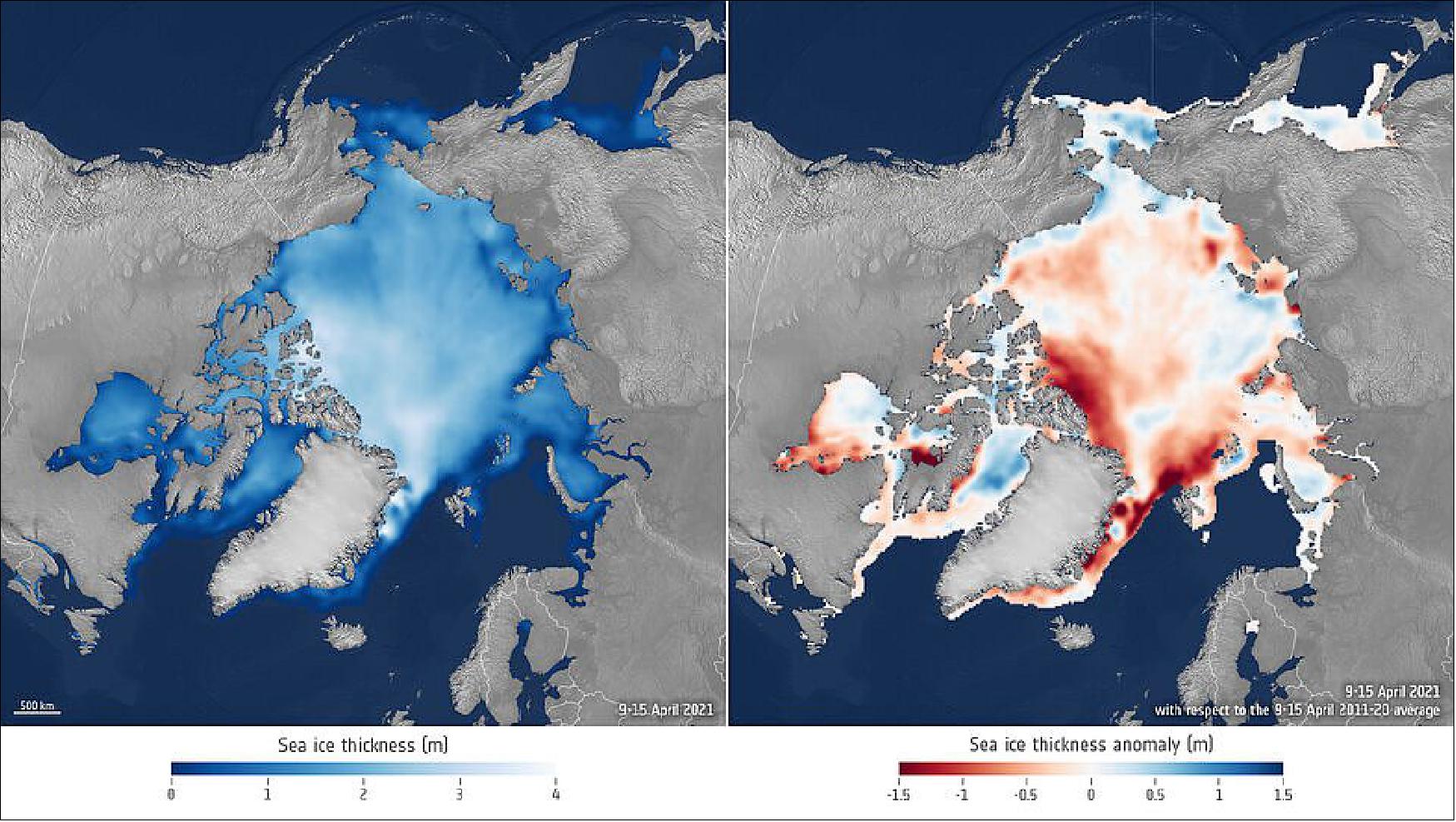
- As well as being used for forecasts, these combined data show that the volume of sea ice in the 2020-21 winter season was at its lowest since these sea-ice data products began in 2010.
- Stefan Hendricks from AWI said, "The driver of this low volume of sea ice is the region north of Greenland and the Canadian Archipelago, where the thickest ice usually resides. Last winter, thick sea ice was almost absent. The rest of the Arctic sea ice is a mix of above and below average."
- The information can also potentially improve forecasts of the weather and climate.
- Many seasonal forecasting centers provide dynamic predictions of sea ice. While assimilating sea-ice concentration is common, constraining initial conditions of sea-ice thickness is in its early stages. However, first assimilation studies at the European Centre for Medium-Range Weather Forecasts (ECMWF) indicate a significant improvement in the seasonal forecast system.
- Beena Balan Sarojini from ECMWF said, "Our results demonstrate the usefulness of new sea-ice observational products in both data assimilation and forecasting systems, and they strongly suggest that better initial sea-ice thickness information is crucial for improving sub-seasonal to seasonal sea-ice forecasts."
• April 19, 2021: The winners of the first ESA-EGU (European Geosciences Union) Excellence Award were awarded their prizes earlier today at the virtual EGU General Assembly ceremony, attended by ESA's Director General, Josef Aschbacher and ESA's Acting Director of Earth Observation Programs, Toni Tolker-Nielsen. 32)
- In late 2020, ESA and the European Geosciences Union (EGU), opened a competition for two awards in Earth observation excellence. The awards are aimed towards researchers in the early phases of their career who have made an outstanding contribution to the innovative use of Earth observation data primarily from European satellites. Two types of awards were advertised: a team and an individual award.
- Following the nomination and selection process, a panel of high-standing Earth observation scientists reviewed the 40 nominations and judged the nominees according to the following categories: excellence in science, excellence in innovation, impact in the field of Earth observation and potential for future Earth observation contributions.
- ESA and EGU are delighted to announce Benoit Meyssignac, a scientist working in the field of oceans remote sensing and geodesy, as the winner of the individual award. Benoit Meyssignac is an internationally renowned expert in the development and analysis of satellite altimetry and space gravimetry observations to tackle fundamental climate science questions.
- Benoit has co-authored more than 60 publications in peer-reviewed journals with more than 3700 citations. He participated in the recent Intergovernmental Panel on Climate Change (IPCC) report as lead author of the sea level chapter of the Special Report on the Ocean and Cryosphere in a Changing Climate (SROCC), contributing author of the polar chapter of the SROCC report and reviewer of the Sixth Assessment Report (AR6).
- Benoit Meyssignac commented, "During the past ten years, my team and I have been able to show that space geodetic measurements from satellite altimetry and satellite gravimetry allows quantification with unprecedented precision of the ocean components of the climate water-energy cycle. This work paves the way for the use of sea level and geodetic remote sensing to provide a new constraint on the Earth's radiation budget and climate sensitivity. This award is timely to highlight these promising results. I am very happy to receive it and I will share it with my team."

- Starting from the pioneering studies on the assimilation of satellite soil moisture products into hydrological modelling, the team has also developed innovative methods to estimate rainfall and irrigation from soil moisture data. The team's work in recent years has demonstrated the potential of satellite products as a crucial support to the hydrological community in improving flood forecasting systems, drought and landslide prediction, and estimating river flow in natural channels.
- Angelica Tarpanelli, researcher at the Italian National Research Council, commented, "Vast regions of the world lack the data needed to predict water supply. With our work, we are unlocking the unprecedented potential of Earth observation to solve this problem. Earth observation can solve the outstanding challenge of hydrologic prediction in data scarce regions, and our research is addressing the target."
- ESA's Acting Director of Earth Observation Programs, Toni Tolker-Nielsen, said, "Today's awardees are young and are at the beginning of their career. The awards will give them the opportunity to make their work more visible to the community, allowing to push new technologies and innovations in Earth observation in a wider context.
- "We would like to congratulate you on this extraordinary recognition. We are sure that you will continue to pioneer European Earth observation scientific achievements in the future and that we will hear from you again!"
- The winners were awarded with free entry to the next in-person EGU General Assembly, as well as travel and expenses, set to take place in 2022.
• December 14, 2020: Hidden from view by ice kilometers thick, there is a vast network of lakes and streams at the base of the Antarctic ice sheet. This subsurface meltwater affects the speed with which the ice sheet flows towards the ocean. Using a decade of altimetry data from ESA's CryoSat satellite, scientists have made an unexpected discovery about how lakes beneath Thwaites glacier have drained and recharged in quick succession. 33)
- Meltwater at the underbelly of the ice is not only a result of frictional heating as the ice flows over the bedrock, but also from heat, called geothermal heat, coming from below the bedrock. Measures of geothermal heat flux in Antarctica are particularly difficult to obtain, and there are large differences between the various current estimates.
- Meltwater under the ice can therefore indicate the state of the bedrock and the degree of geothermal flux. This is important because they both affect the speed the ice flows and drains into the ocean.
- When this basal melt water reaches the ocean it forms buoyant meltwater plumes, which drive an under-ice circulation that brings warm deep ocean water into contact with the ice and causing the ice to melt even more.
- Although this subglacial network is hidden from view by kilometers-thick ice, the movement of meltwater deep below causes tiny movements on the surface of the ice, which, remarkably, can be detected and monitored from space.
- At around 120 km wide, Thwaites is the largest glacier on Earth and one of the most fragile glaciers in Antarctica. It is, therefore, the subject of much international research through the UK National Environment Research Council NERC/US National Science Foundation (NSF) International Thwaites Glacier Collaboration and ESA's 4D Antarctica project.
- ESA's Diego Fernandez, head of the Earth Observation Science Section and overseeing the 4D Antarctica project, said, "The project draws together several years of research from different teams to form a new comprehensive assessment of Antarctic ice-sheet hydrological processes – from the lithosphere and subglacial environment to surface-melting process.
- "This will certainly contribute to establishing a robust scientific base on which to develop a Digital Twin of Antarctica in the future."
- Using more than 10 years' worth of altimetry data from ESA's CryoSat satellite, scientists have discovered that the lakes beneath Thwaites, the largest of which is over 40 km long, drained in quick succession, in 2013 and then in 2017.
- This kind of reoccurring drainage under Thwaites has never before been recorded.
- Scientists estimate that the rate of drainage peaked at about 500 m3/s – possibly the largest outflow of meltwater ever reported from subglacial lakes in this region.
- This peak rate is about eight times faster than the River Thames in England discharges on average to the North Sea.
- George Malczyk, lead author from the University of Edinburgh in the UK, said, "We used CryoSat to show a period of lake activity only four years after the previous drainage event in 2013.
- "But what is interesting about this second drainage event is how different it is from the first, with a faster transfer of water and increased water discharge. Our observations highlight that there were potentially significant modifications to the subglacial system between these two events."
- Between 2013 and 2017, the scientists can see that the lakes recharged.
- Linking these observations with basal meltwater flowing into the lake through a network of basal channels, gave for the first time, an estimate of the rate of melting at the base of the ice sheet. By comparing these rates to modelled estimates, the scientists were able to demonstrate that models underestimate basal melting under this region of Thwaites by nearly 150%.
- These findings will help to assess and constrain models and, in turn, improve the representation of the ice sheet system, and better project its evolution.
- Noel Gourmelen, also from the University of Edinburgh, said, "What takes place under the ice sheet is critical to how it responds to changes in the atmosphere and ocean around Antarctica, and yet it is hidden from view by kilometers of ice which makes it very difficult to observe.
- "This movement of water give us a glimpse of where the water is and how much and how fast it moves across the system. Together this is key information about the nature of the subglacial environment and the processes of the hydrological network under the ice sheet. These findings provide key information that can help us project how the ice sheet adds to sea level as it responds to climate change.
- "Being able to monitor these remote regions from space over long periods of time is extremely important. As such, the planned CRISTAL (Copernicus Polar Ice and Snow Topography Altimeter) mission, which is part of the expansion of Europe's Copernicus program, will be crucial. It will ensure continuity and expansion of the current capabilities to study the entire ice sheet from space."
- Dr Fernandez added, "With this activity we want to contribute to the scientific efforts undertaken by the NERC/NSF International Thwaites Glacier Collaboration and by the EU Polar Cluster, to better understand and predict the dramatic changes affecting the polar regions. It is only through scientific collaboration, both within Europe and internationally, that we will be able to collectively address the major scientific and societal challenges we all face."
• December 9, 2020: Celebrating 200 years since the discovery of the Antarctic continent, the UK Committee for Antarctic Place-Names has named 28 mountains, glaciers and bays after modern-day scientists who have advanced our understanding of this remote continent. Four of the names on the list have strong links to ESA, having either worked on the development of polar-orbiting altimetry missions such as ERS-1, ERS-2, Envisat and CryoSat-2, or subsequently by using their data together with other satellite missions for key polar research projects. 34)
- Named in honor of Seymour Laxon, Laxon Bay lies in the northwest of the Antarctic Peninsula. Prof. Laxon was the Director at the Centre for Polar Observation and Modelling at University College London. His research pioneered the use of satellite altimetry to measure the gravity field, sea-ice thickness and surface circulation in the polar oceans. His work provided evidence that enabled the development of the CryoSat mission.
- Named after Katharine Giles, Giles Bay also lies in the northwest of the Antarctic Peninsula. Dr Gilles' research focussed on sea ice, ocean circulation and wind patterns, and the use of satellite altimetry to measure the thickness of Arctic and Antarctic sea ice.
- Both Prof. Laxon and Dr Gilles were instrumental in a number of ESA's polar field experiments to support the CryoSat mission.
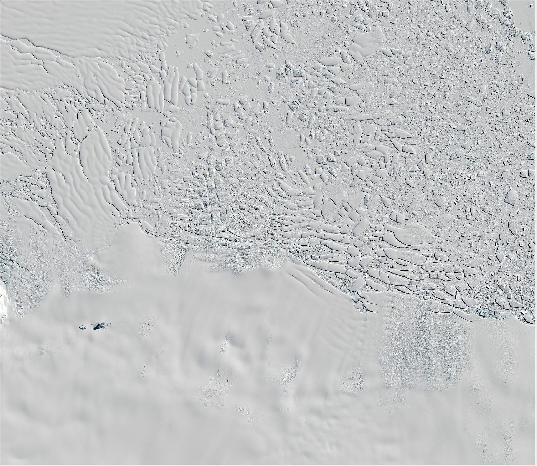
![Figure 25: Laxon Bay lies in the northwest of the Antarctic Peninsula. Laxon Bay is about 10 km wide and 3 km deep and lies between Palosuo Islands and the west side of Renaud Island, Biscoe Islands. The research of Seymour Laxon pioneered the use of satellite altimetry to measure the gravity field, sea-ice thickness and surface circulation in the polar oceans. His work provided evidence that enabled the development of the CryoSat mission. Giles Bay also lies in the northwest of the Antarctic Peninsula. Giles Bay is about 4 km wide and 3 km deep and lies between Weaver Point and Tula Point at the northern end of Renaud Island, Biscoe Islands. Katharine Gilles' research focussed on sea ice, ocean circulation and wind patterns, and the use of satellite altimetry to measure the thickness of Arctic and Antarctic sea ice [image credit: CPOM (Center for Polar Observation and Modelling), located at the University of Leeds]](https://www.eoportal.org/ftp/satellite-missions/c/CryoSat2_220722/CryoSat2_Auto47.jpeg)
- Jonathan Bamber is currently Professor of Physical Geography at the University of Bristol and now has Bamber Glacier on Adelaide Island named in his honor. Prof. Bamber is a specialist in using satellite altimetry to study the morphology and dynamics of the Antarctic and Greenland ice sheets and ice shelves, and the contribution of land ice to sea-level change.
- ESA's Mark Drinkwater said, "The scientific advances made by the UK scientists Seymour Laxon, Catherine Giles and Jonathan Bamber using satellite altimetry data have been ground breaking and pivotal for ESA. Each added successive layers to our understanding of how polar ice and the polar oceans respond to climate change. Their respective contributions are unique, and have led to the success of ESA's dedicated polar-orbiting ice mission CryoSat."
- CryoSat-2 has now been in orbit for well over 10 years measuring variations in the height of Earth's ice to reveal how climate change is affecting the polar regions. It has contributed to the recent worrying findings that Greenland and Antarctica are now losing ice six times faster than in the 1990s, which has clear implications for future sea-level rise. Information such as this is vital for international policy making in responding to climate change.
- Fricker Ice Piedmont, on the eastern side of Adelaide Island, honors Helen Fricker. Prof. Fricker is the founder and co-lead of Polar Center at Scripps Institution of Oceanography, UC San Diego, California. She too has played an important scientific role in ESA's ERS, Envisat and CryoSat missions. As glaciologist and current science team member on NASA's ICESat and ICESat-2 missions she has worked on Antarctic ice shelf evolution and change detection, and Antarctic subglacial hydrology. More recently, she also worked on the project that involved synchronizing CryoSat's orbit with that of ICESat-2 so that scientists can benefit from simultaneous measurements and from the synergy between these different space sensors.
- ESA's CryoSat mission manager, Tommaso Parrinello, said, "It's wonderful to see that these scientists, who have contributed so much to CryoSat, now have their names forever in Antarctica.
- "The development of CryoSat started many years ago when Seymour Laxon was instrumental in its conception. The mission continues to amaze us by returning fantastic science. We are just now looking into the findings of having CryoSat and ICESat-2 aligned in orbit, and here we also have Helen Fricker to thank for the part she has played in this important change."
- The new names will feature on all British maps, charts and publications and are being put to the Scientific Committee on Antarctic Research for inclusion in its international directory, which should lead to all other nations using the names, too.
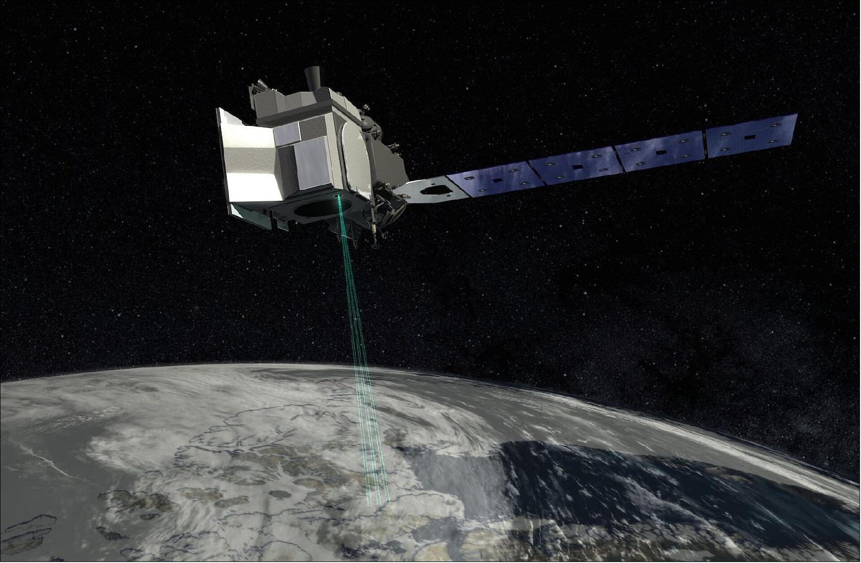
• August 3, 2020: Ice plays a critical role in keeping Earth's climate cool, but our rapidly warming world is taking its toll and ice is in general decline. For more than 10 years, ESA's CryoSat-2 has been returning critical information on how the height of our fragile ice fields is changing. Nevertheless, to gain even better insight, ESA has spent the last two weeks nudging CryoSat-2 into a higher orbit to synchronize it with NASA's ICESat-2 so that scientists can benefit from simultaneous measurements from different space sensors. 35)
- CryoSat-2 carries a radar altimeter and NASA's ICESat-2 carries a laser. Both instruments measure the height of ice by emitting a signal and timing how long it takes the signal to bounce off the ice surface and return to the satellite. Knowing the height of the ice allows scientists to calculate its thickness.
- However, snow can build up on top of the ice and can hide the ice's true thickness.
- While CryoSat's radar penetrates through the snow layer and reflects closely off the ice below, ICESat-2's laser reflects off the top of the snow layer. Blending simultaneous satellite laser and radar readings means that snow depth can be measured directly from space for the first time.
- Knowing the depth of the overlying snow will improve the accuracy of sea-ice thickness measurements and improve our knowledge of how snow and ice surfaces, with different physical properties, scatter back the signal from the instruments.
- ESA's CryoSat-2 mission manager, Tommaso Parrinello, says, "The idea of having CryoSat-2's orbit align with that of NASA's ICESat-2 goes back some years now. It has taken a lot of planning and is a significant undertaking, something we haven't done before.
- Aligning CryoSat-2 with ICESat-2 is like having one satellite with two instruments."
- ICESat-2 orbits at an altitude of around 500 km and CryoSat used to orbit an altitude of around 720 km.
- Two weeks ago, flight operators at ESA's spacecraft operation center in Germany began gently firing CryoSat's thrusters to raise its orbit by almost 1 km to bring it into synch with ICESat-2.
- Ignacio Clerigo, ESA's CryoSat spacecraft operations manager, explained, "CryoSat-2 orbit was much higher and slower than ICESat-2, so we couldn't align them by having them orbit in tandem. Instead, we raised CryoSat-2 by 900 m through a series of 15 precisely timed thruster burns. The two satellites will now overlap every 19th orbit of CryoSat and 20th orbit of ICESat-2."
- Since sea ice floats in the ocean, currents and wind move it around. Under normal circumstances, the two satellites would take measurements over the same location a number of hours apart, so it could be different ice under their normal orbital paths.
- Dr Parrinello continued, "By raising CryoSat-2's orbit we find this sweet spot where every 1.5 days the two satellites will pass over areas of the polar regions around the same time. These few minutes of almost coincident measurements will be key for studying sea ice. CryoSat-2 will remain in this orbit now until the mission is over."
- Josef Aschbacher, ESA's Director of Earth Observation Programs, remarked, "Having both agency's satellites aligned in orbit is a wonderful example of our organizations working together to bring greater benefits to science. These coincident measurements are going to be very important for scientists studying our changing world."
- Sea ice plays an important role in the global climate. For example, it helps maintain Earth's energy balance while helping keep polar regions cool by reflecting incident sunlight back into space. It also keeps the air cool by forming an insulating barrier between the cold air above and the warmer ocean water below.
- This new information could help improve climate models, particularly for Antarctica. The models scientists currently use to gauge snow depth when calculating sea ice work reasonably well for the Arctic, but less so for the Antarctic.
- It could also help tackle the difficult task of measuring sea ice in summer. In warmer weather, ponds of meltwater on the ice swamp the signal from CryoSat-2, but ICESat-2 has the precision to detect these ponds and differentiate between them and the breaks between floes of ice.
• April 8, 2020: Today marks 10 years since a Dnepr rocket blasted off from an underground silo in the remote desert steppe of Kazakhstan, launching one of ESA's most remarkable Earth-observing satellites into orbit. Tucked safely within the rocket fairing, CryoSat had a tough job ahead: to measure variations in the height of Earth's ice and reveal how climate change is affecting the polar regions. Carrying novel technology, this extraordinary mission has led to a wealth of scientific discoveries that go far beyond its primary objectives to measure polar ice. And, even at 10 years old, this incredible mission continues to surpass expectations. 36)
- The launch of a satellite is always a time to hold your breath, but CryoSat's liftoff on 8 April 2010 was arguably more tense than most as it came less than five years after the original satellite was lost owing to a rocket malfunction.
- So important was the need to understand what was happening to Earth's ice, the decision to rebuild was taken quickly – and thankfully, this day 10 years ago heralded the beginning of a mission that was set to advance polar science like no other.
- While other satellite missions can measure changes in the extent of Earth's ice, CryoSat completes the picture by recording changes in ice height, which are used to work out changes in thickness and volume – key to understanding the total amount of ice loss.
- CryoSat was designed to observe two types of ice: the vast ice sheets of Antarctica and Greenland that rest on land, and the sea ice floating in the polar oceans.
- Not only do these two forms of ice have different consequences for our planet and climate, but they also pose different challenges when trying to measure their thickness.
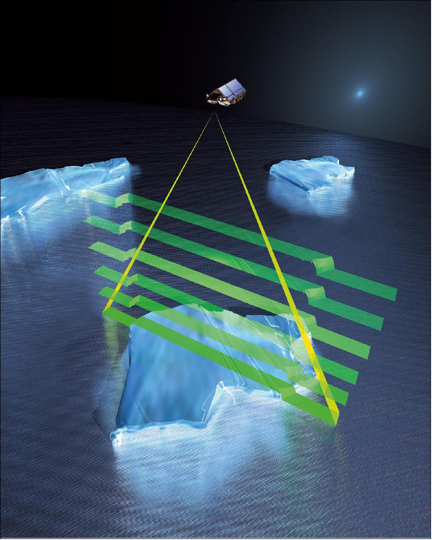
- To do this, CryoSat carries the first spaceborne synthetic aperture interferometric radar altimeter, a sensor optimized to detect sea-ice floes as they drift in the ocean and to study the rugged glaciers that drain the polar ice sheets.
- In addition, CryoSat's orbit reaches latitudes of 88° North and South, which takes it closer to the poles than all previous polar-orbiting altimetry satellites.
- ESA's Director of Earth Observation Programs, Josef Aschbacher, said, "CryoSat is the epitome of an ESA Earth Explorer. It uses completely new technology to fill gaps in our scientific knowledge. The issue of diminishing ice linked to climate change is a real concern, and over the last 10 years this mission has been a game changer.
- Andrew Shepherd from the University of Leeds, UK, added, "CryoSat's contribution to polar science is truly astonishing. Not only do we now have a clear picture of how much ice Earth is losing, but its measurements have helped to improve the models we use to predict future climate change – information that is critical for society to adapt."
- CryoSat has also revealed how the world's 200,000 mountain glaciers have succumbed to climate change, thanks to advanced swath processing of its radar measurements, which allows small regions to be mapped in fine detail. This new technique takes the mission beyond its brief to study polar ice alone.
- Although changes in sea ice do not affect sea level directly because it is afloat, it plays a central role in the global climate system as it reflects solar radiation back into space, and because it moderates ocean heat transport around the planet by insulating the relatively warm water from the cold polar air. CryoSat has been instrumental in mapping changes in the thickness and volume of Arctic sea ice.
- Prof. Shepherd added, "Despite the long-term decline in the extent of Arctic sea ice, there have been significant year-to-year fluctuations in its thickness, and its volume has fallen in only seven of the past 10 years. But even with a decade of CryoSat measurements, the seasonal cycle of sea-ice growth and decay is still too large to confidently detect a long-term trend in volume, and so continued observation is essential.
- As well as fulfilling its primary role as a polar ice mission, CryoSat's measurements have been put to good use in a wide range of alternative and innovative applications. During the winter, CryoSat has been able to record changes in the thickness of ice on lakes, and in the summer it has been used to monitor lake and river water levels across the globe – information that is important for travel and fishing, for example.
- CryoSat's measurements are now an important reference of global sea level in the polar regions and beyond, thanks to its high-inclination orbit and long-repeat cycle, allowing scientists to refine the long-term trend and to detect short-term fluctuations associated with ocean dynamics.
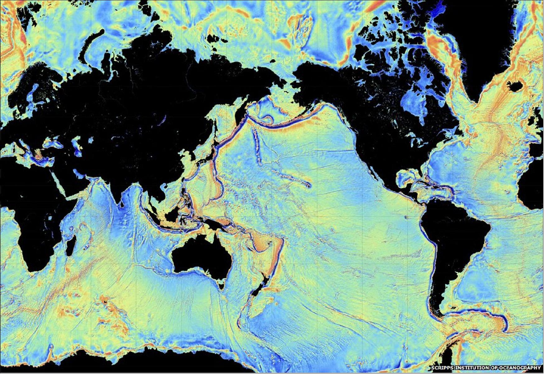
- And, it has even revealed what lies beneath the ocean surface thanks to its ability to detect tiny changes in marine gravity, which reflect the shape of the sea bed. CryoSat's bathymetric charts are now an important tool for studying ocean dynamics, currents and tides, as well as for ship safety.
- ESA's CryoSat Mission Manager, Tommaso Parrinello, said, "These are just some of CryoSat's outstanding results and the mission is still going strong, but we will focus more on this at the CryoSat anniversary conference, which we've had to postpone until October because of the COVID-19 pandemic. In the meantime, however, I cannot praise the mission and all the people who have worked on it enough."
- ESA's Mark Drinkwater added, "Indeed, CryoSat is still giving us incredible data to advance science, and with its new synthetic aperture radar and interferometric capabilities it has also laid the foundation for the Copernicus Polar Ice and Snow Topography Altimeter (CRISTAL) operational mission, which we are now developing on behalf of the ESA Member States and the European Commission."
- CRISTAL will fill the recognized gap in sustained long-term monitoring of polar ice variability for the Copernicus Climate Change Service and Copernicus Marine Environment Monitoring Service, maritime security and international ice charting, and in support of the EU Integrated Arctic Policy and commitments to the Paris Agreement and Green New Deal.
• January 27, 2020: Ice loss from Pine Island Glacier has contributed more to sea-level rise over the past four decades than any other glacier in Antarctica. However, the way this huge glacier is thinning is complex, leading to uncertainty about how it is likely to raise sea level in the future. Thanks to ESA's CryoSat-2 mission, scientists have now been able to shed new light on these complex patterns of ice loss. 37)
- Although Pine Island Glacier is one of the most intensively and extensively investigated glacier systems in Antarctica, different model projections of future mass loss give conflicting results; some suggesting mass loss could dramatically increase over the next few decades, resulting in a rapidly growing contribution to sea level, while others indicate a more moderate response.
- Identifying which is the more likely behavior is important for understanding future sea-level rise and how this vulnerable part of Antarctica is going to evolve over the coming decades.
- In a paper published in Nature Geoscience, scientists from the University of Bristol, UK, describe how they used information from CryoSat to help clarify the situation. They discovered that the pattern of ice loss is evolving in complex ways, both in space and time.
- Rates in the fast-flowing central trunk of the glacier have decreased by about a factor of five since 2007 – and this is the opposite of what was observed prior to 2010.
- These new results suggest that rapid migration of the grounding line, the place where the grounded ice first meets the ocean, is unlikely over the next decades, without a major change in the role of the ocean in ice loss. Instead, the results support model simulations that imply that the glacier will continue to lose mass, but not at much greater rates than present.
- Lead author Prof. Jonathan Bamber from the University of Bristol's School of Geographical Sciences, said, "This could seem like a ‘good news story', but it's important to remember that we still expect this glacier to continue to lose mass in the future and for that trend to increase over time, just not quite as fast as some model simulations suggested.
- "It's really important to understand why the models are producing different behavior in the future and to get a better handle on how the glacier will evolve with the benefit of these new observations.
- "In our study, we didn't make projections, but with the aid of these new data we can improve model projections for this part of Antarctica."
- Tommaso Parrinello, ESA's CryoSat mission manger, added, "In April, CryoSat will have been in orbit for 10 years, far exceeding its expected life. We continue to be proud of the contribution to science this extraordinary satellite mission is making.
- "And here, with the issue of sea-level rise a major global concern, the better equipped we are with facts the better it is. CryoSat has helped clarify the situation at Pine Island Glacier, which is not only important for our scientific understanding, but ultimately for society at large."
• December 13, 2019: It is now almost 10 years since ESA's CryoSat-2 mission was launched. Throughout its decade in orbit, this novel satellite, which carries a radar altimeter to measure changes in the height of the world's ice, has returned a wealth of information about how ice sheets, sea ice and glaciers are responding to climate change. One of the most recent findings from this extraordinary mission shows how it can be used to map changes in the seaward edges of Antarctic ice shelves. 38)
- About three-quarters of the Antarctic coastline consists of ice shelves. They are permanent floating extensions of the ice sheet that are connected to and fed by huge ice streams draining the interior ice sheet. Ice shelves form as the ice sheet flows towards the ocean and detaches from the bedrock beneath. The advance or retreat of ice shelves is determined by a balance between mass gain from the flow of ice behind and snowfall on top, and mass loss through ocean melting at the base or iceberg calving at the edge.
- Ice shelves are important for the stability of the ice sheet because they act as buttresses, holding back the glaciers that feed them and slowing the flow of land ice into the ocean that contributes to sea-level rise.
- However, in recent years warming ocean waters and higher air temperatures are taking their toll on some of the ice shelves, causing them to thin, shrink or even collapse entirely. Therefore, mapping ice-shelf calving front locations is important for understanding and predicting future changes in the stability of the ice sheet.

- A paper published recently describes how scientists have developed a novel approach of using CryoSat to generate a unique time series of ice front positions for the Filchner-Ronne ice shelf – the second largest ice shelf in Antarctica. 39)
- Jan Wuite, from ENVEO (Environmental Earth Information Technology GmbH) in Austria, said, "The detection of the calving front is based on the premise that the edge of an ice shelf is typically a steep ice cliff, with a drop of tens of meters to the ocean surface or sea-ice cover, which is clearly revealed by CryoSat.
- "Applying a new method, called ‘elevation edge', to CryoSat's data has revealed that the entire Filchner-Ronne ice shelf advanced by more than 800 km2 per year between 2011 and 2018. The growth of the ice shelf was only interrupted by the calving of a 120 sq km iceberg in 2012 and a few smaller-scale events."
- Eventually, the advancing ice front is expected to break off as part of the natural ice shelf cycle, but these are rather episodic events that only happen every few years or sometimes decades. Many questions still need to be answered as to what is driving these calving events.
- Thomas Nagler, also from ENVEO, added, "Combining this new dataset with ice velocities derived from Copernicus Sentinel-1 data allows us to calculate changes in the thickness and area of the ice shelf, as well as the advance rates and iceberg calving rates, emphasizing the value of combining data from both satellite missions."
- ESA's Mark Drinkwater noted, "Understanding how the world's ice shelves are changing is fundamental to assessing ice sheet stability, and the role of ice shelves in controlling ice-sheet contribution to sea-level rise."
- "Just this week a paper was published in Nature stating that the Greenland ice sheet mass loss closely follows the IPCC high-end climate warming scenario – and the research was based on measurements from a number of different satellites.
- "Here, we see how using this innovative elevation edge method with CryoSat data is a welcome addition to standard calving front location detection techniques based on radar and optical satellite imagery. This is great news, as the more information we have the more confident we can be about what's going on in the far reaches of the polar regions."
- The new method provides calving front locations at regular intervals and can fill existing gaps in time and space. Moreover, it simultaneously provides ice-thickness measurements that are needed to calculate mass changes, and it also has a high degree of automation which removes the need for heavy manual intervention.
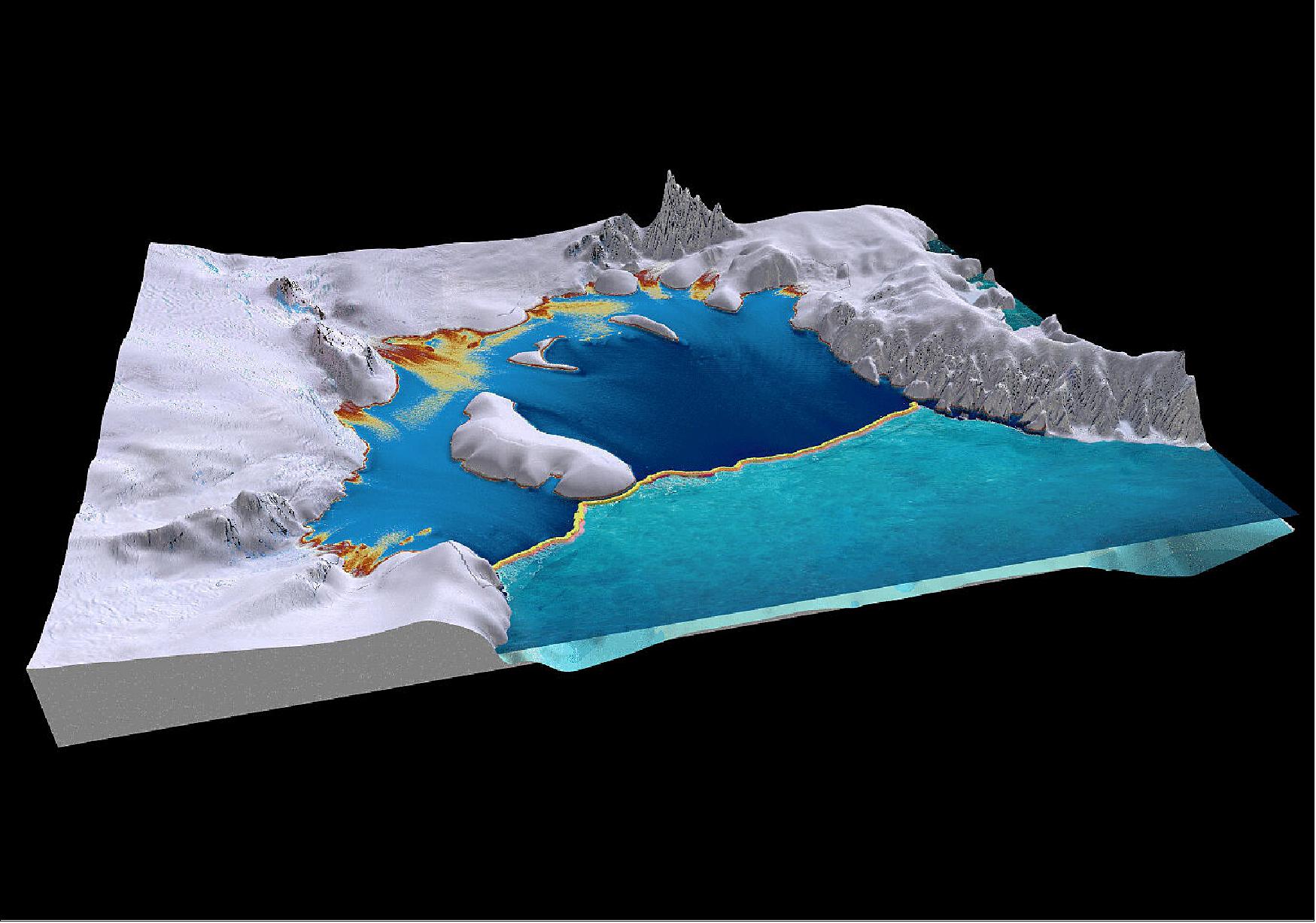
- Dr Wuite added, "We fully expect that, in the future, altimetry data will deliver a systematic and continuous record of change in ice-shelf calving front positions around Antarctica.
- "With CryoSat set to remain in service and the future CRISTAL Copernicus Polar Ice and Snow Topography Altimeter mission – one of the Copernicus high-priority candidate missions – on the table for development, there are certainly excellent opportunities for satellite radar altimetry to deliver valuable new calving front location datasets to monitor the effects of climate change in Antarctica."
• August 5, 2019: The rapidly changing climate in the Arctic is not only linked to melting glaciers and declining sea ice, but also to thinning ice on lakes. The presence of lake ice can be easily monitored by imaging sensors and standard satellite observations, but now adding to its list of achievements, CryoSat-2 can be used to measure the thickness of lake ice – another indicator of climate change. 40) 41)
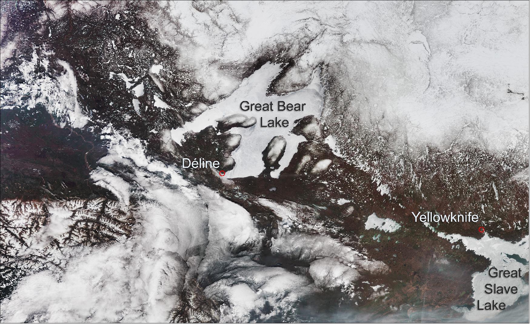
- CryoSat-2, one of ESA's Earth Explorer satellites, carries the first radar altimeter of its kind. The instrument is traditionally used to determine the thickness of sea ice floating in oceans and to monitor changes in vast ice sheets on land, providing evidence of Earth's diminishing polar ice.
- Lakes in North America's Arctic and sub-Arctic regions cover between 15% and 40% of the landscape, and play an important role in the region's climate. They are also a vital resource for both society and an important habitat for aquatic wildlife.
- Used as a platform for activities such as fishing, hunting and travel, knowledge of ice thickness is important for assessing safety. Monitoring changes in water volume and levels are also important for the supply of water for domestic, commercial and industrial use.
- For the first time, CryoSat-2's altimeter has been used to measure the thickness of ice in the Great Slave Lake and the Great Bear Lake, in the Northwest Territory of Canada. Scientists from the University of Alberta and York University have documented their findings in a paper published in the Institute of Electrical and Electronics Engineers Transactions on Geoscience and Remote Sensing.
- The Great Slave Lake and the Great Bear Lake were chosen for their flat and smooth icy surfaces, and scientists were able to distinguish radar reflections from both ice-free and ice-covered areas. By subtracting the travel times of the radar signals between the ice surface and ice bottom, they were able to measure the thickness of the ice floating on the lake.
- The distance between the two reflections increased during winter, representing the seasonal thickening of the lake ice, and were then accurately validated with in situ drill-hole measurements.
- Christian Haas from the University of Bremen (formerly at York and Alberta), said, "Thanks to CryoSat-2, we are able to study seasonal changes and cycles of ice thickness, as well as volume and variability for many other smaller lakes in the sub-Arctic.
- "Although we have chosen to study the two largest lakes in the region, the same method can be applied to many other smaller lakes.
- "In addition to monitoring ice thickness, the method could also be used to retrieve lake water levels and volume throughout winter."
- Jerome Bouffard, CryoSat-2's data quality manager, says "We are delighted to see such results coming from CryoSat-2. Its data can provide key information over multiple surfaces that are critical to scientists' understanding of the role that ice plays in the Earth system, at both local and global scales."
• July 24, 2019: Our knowledge of the depth and shape of the Arctic Ocean floor – its bathymetry – is insufficient. Owing to year-round sea-ice coverage and the cost of research in this remote region, much of the Arctic Ocean's bathymetry has remained a mystery, until now. 42)
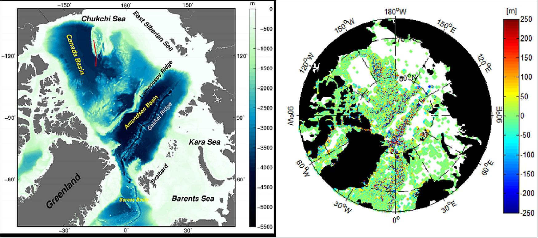
- Bathymetry maps are crucial for studying ocean dynamics, currents and tides, as well as for ship safety. Several campaigns to map seafloor bathymetry through ship soundings have been proposed, but only small fractions of the Arctic Ocean have ever been covered.
- Scientists from DTU Space, Denmark's national space research institute, have published a paper that reveals the first Arctic bathymetry map using marine gravity. 43)
- The surface of the ocean is not flat. Because of gravitational pull, the height of the ocean surface mimics the rise and fall of the ocean floor. Areas of greater mass such as underwater mountains have a higher gravity and therefore attract more water creating a rise in the sea surface.
- Fine-tuning the relationship between bathymetry and gravity in the Arctic Ocean has enabled scientists to calculate sea—floor bathymetry from satellite gravity measurements.
- By using ERS-1 and ERS-2, Envisat and seven years' of CryoSat data, an altimetric gravity model has been developed by DTU Space. This has been combined with the existing IBCAO bathymetry map to create a new and improved hybrid bathymetry map of the Arctic Ocean.
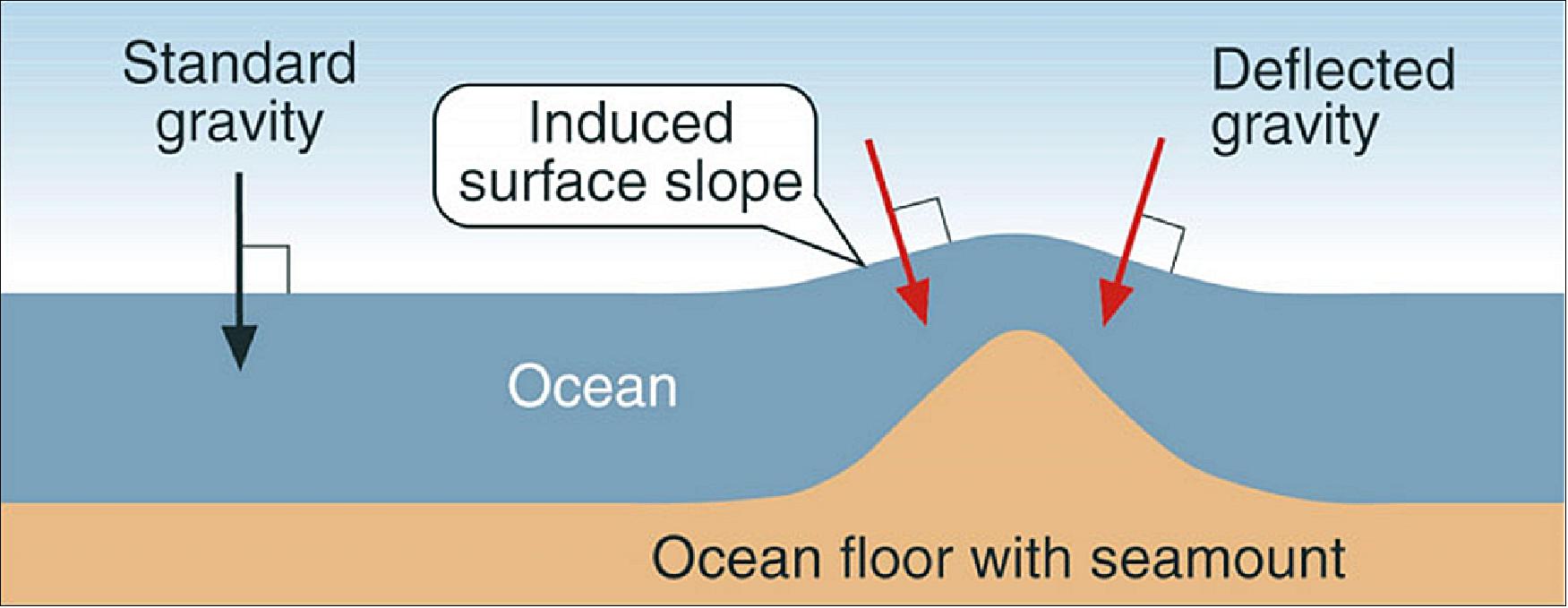
- Fine-tuning the relationship between bathymetry and gravity in the Arctic Ocean has enabled scientists to calculate sea—floor bathymetry from satellite gravity measurements.
- By using ERS-1 and ERS-2, Envisat and seven years' of CryoSat-2 data, an altimetric gravity model has been developed by DTU Space. This has been combined with the existing IBCAO bathymetry map to create a new and improved hybrid bathymetry map of the Arctic Ocean.
- CryoSat-2 was originally launched to measure sea-ice thickness, but data from the Earth-observing satellite have been exploited for other studies. Carrying a radar altimeter, the satellite can sense the gravity field at the ocean surface, so that seafloor characteristics are revealed – allowing it to map the global marine gravity field at a high spatial resolution.
- "The existing IBCAO (International Bathymetric Chart of the Arctic Ocean) bathymetry map of the Arctic Ocean is based purely on ship soundings and assisted by digital depth contours. Combining the IBCAO bathymetry with altimetry-derived marine gravity has resulted in a more accurate bathymetry map of the Arctic," says Ole Baltazar Andersen from DTU Space.
- He continues, "The true value in the satellite data lies in the fact that it can help fill in data gaps between ship soundings, giving us a more complete picture of the Arctic bathymetry."
- The value of the hybrid bathymetry has also been validated using recent independent ship sounding surveys accessed through the NOAA's National Center for Environmental Information (NCEI). Over the Chukchi Cap in the Canadian Arctic, the hybrid bathymetry could improve the existing IBCAO model derived from sparse ship tracks in the region.
- "This mapping shows our satellites' capability of providing us with new data, especially in more difficult areas such as the unknown Arctic waters," says Jérôme Benveniste, senior advisor at ESA.
- Josef Aschbacher, ESA's director of Earth observation programs, added, "And this is yet another piece of the jigsaw that adds to our understanding of the planet – and critically this kind of information can be used for maritime safety therefore benefiting society."
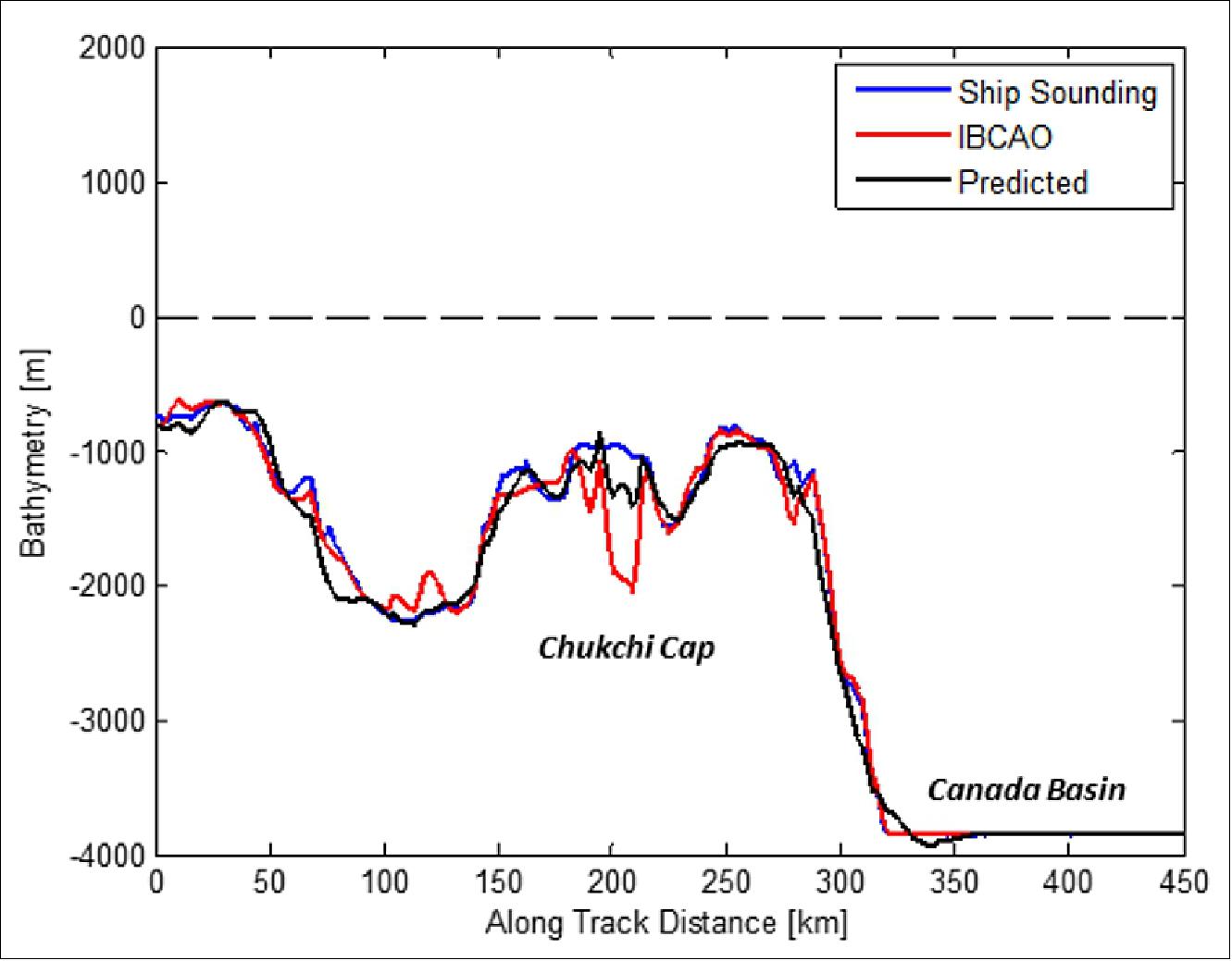
• July 11, 2019: We are all aware of the ebb and flow of the tide every day, but understanding tidal flow is important for a range of maritime activities and environmental monitoring, such as search and rescue operations, shipping routes and coastal erosion. The Arctic Ocean tides are particularly difficult to understand, but a new tidal model produced using ESA satellite data may shed some light on what is happening in this remote area. 44)
- In many areas of the ocean, direct in situ measurements of ocean tides are rare. This means that tidal models need to be developed to fill in the gaps in observations.
- Owing to its location, the Arctic Ocean proves more difficult because of the scarcity of in situ observations, the frequent presence of sea ice and poorly-documented bathymetry. The bathymetry, or the depth and shape of the ocean floor, is crucial for studying ocean dynamics and for ship safety.
- Arctide2017 is a high-resolution tidal atlas of the Arctic Ocean. Developed by NOVELTIS (Labège, France), DTU Space (Lyngby, Denmark) and LEGOS (Toulouse, France), it combines altimeter data from ESA's Envisat and CryoSat-2 satellites into the most complete dataset used in the Arctic region to estimate tidal information. 45)
- Satellite altimetry missions are often used to estimate ocean tide information, however this technique requires a long-time series of satellite data to derive accurate tidal estimates – usually more than 10 years.
- CryoSat-2 is traditionally used to determine changes in the thickness of ice, but its radar altimeter can also measure changes in sea level. Moreover, thanks to its unusually high-inclination orbit that takes it close to the poles, ESA's CryoSat-2 mission can also provide tidal information in regions that are not sampled by other satellite altimetry missions.
- Also the number of altimeter observations increases towards the poles due to how the satellites circle Earth. This allows scientists to estimate tidal information over shorter periods of time, particularly in the Arctic Ocean.
- The Arctide2017 is based on modelling with data assimilation for the main linear tidal components, however non-linear tidal components have not yet been produced – until now.
- Tidal information extracted from satellite altimetry observations are generally reliable only for ‘linear tides,' which describe the tide as the simple result of the gravitational pull of the Moon and Sun.
- However, other factors influence the tides such as bathymetry and coastlines, generating ‘non-linear' tidal components. In shallower waters, a significant part of the tidal signal is due to these ‘non-linear' components – causing very complex tides. One way of estimating these tides is through tidal modelling.
- Mathilde Cancet, a scientific engineer at NOVELTIS comments, "Thanks to the model's grid resolution and the specific processing of the assimilated altimetry observations, the Arctide2017 regional tide atlas outperforms the concurrent regional and global models in most regions of the Arctic Ocean."
- The Arctide tidal model will benefit satellite altimetry sea level measurements in the Arctic Ocean, as well as various end-users such as modelers and other stakeholders in the maritime industry."
- This work was carried out in within the CryoSat Plus for Ocean (CP4O) project funded by ESA.
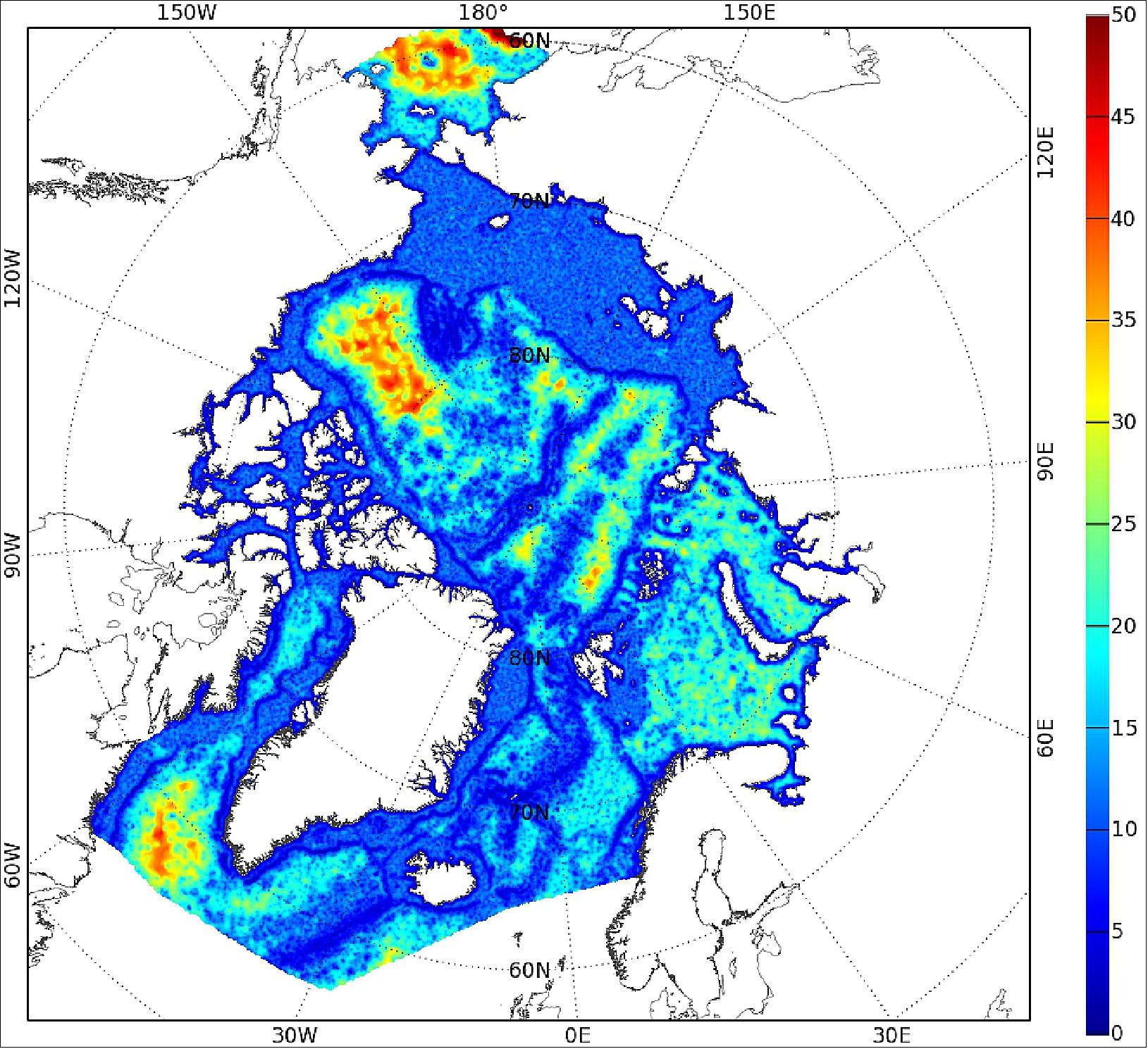
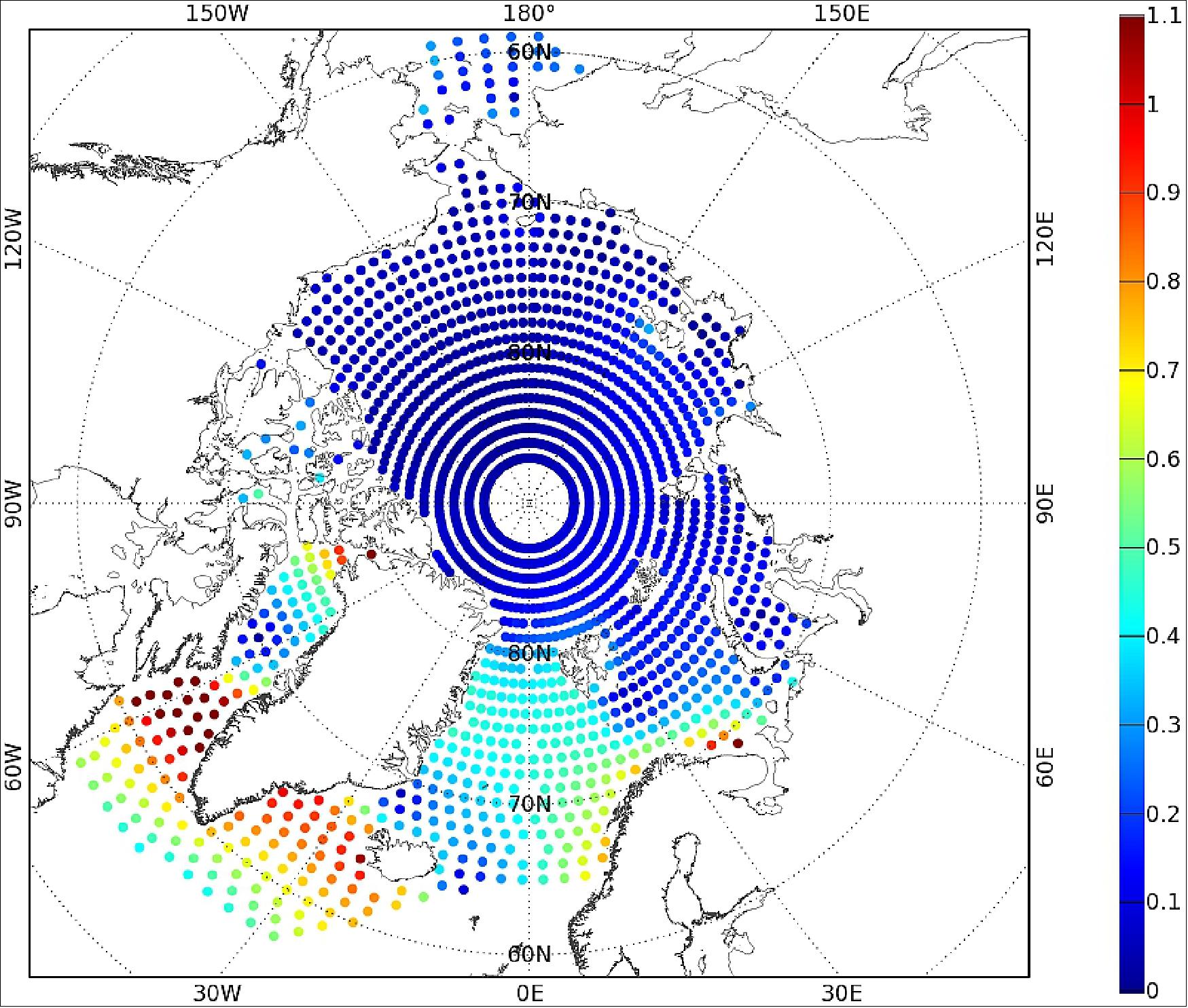
• May 14, 2019: Ice is a hot topic when it comes to understanding and monitoring how this fragile component of the Earth system is being affected by climate change. Scientists, therefore, go to great lengths to study changes happening in the remote icy reaches of our planet – a subject that is being discussed in detail at this week's Living Planet Symposium in Italy. Among the results being presented is a novel 3D dataset of Antarctica. Scientists from the University of Edinburgh, UK, created this new view by processing data from ESA's CryoSat in a clever way. CryoSat carries a radar altimeter that measures the height of the world's ice. Typically, the data are used to map the height of ice at single points. And, since it was launched in 2010, this has revealed much about how ice sheets, glaciers and sea ice are changing. 46)
- The technique is allowing scientists to better understand change and predict how ice sheets, glaciers and ice caps may behave as climate change takes a stronger grip. This is important with respect to global concerns such as sea-level rise.
- The team used this method to map Greenland in 2017, and now the Antarctica model is available. Both datasets can be downloaded from the CryoTop website.
- The CryoTop datasets contain surface elevation generated from swath processing of CryoSat-2 measurement. The CryoTop datasets also contain gridded products generated from the swath derived elevation, these are 2 Digital elevation models (500 m and 1 km posting) and 2 maps of rates of surface elevation change (500 m and 1 km posting) as well as associated errors. The swath elevation data are provided as NetCDF files following the naming convention of the original CryoSat-2 datafiles provided by the European Space Agency, the gridded products are provided as GeoTIFF files. The methodology and data format are described in the dataset user manual. 47)
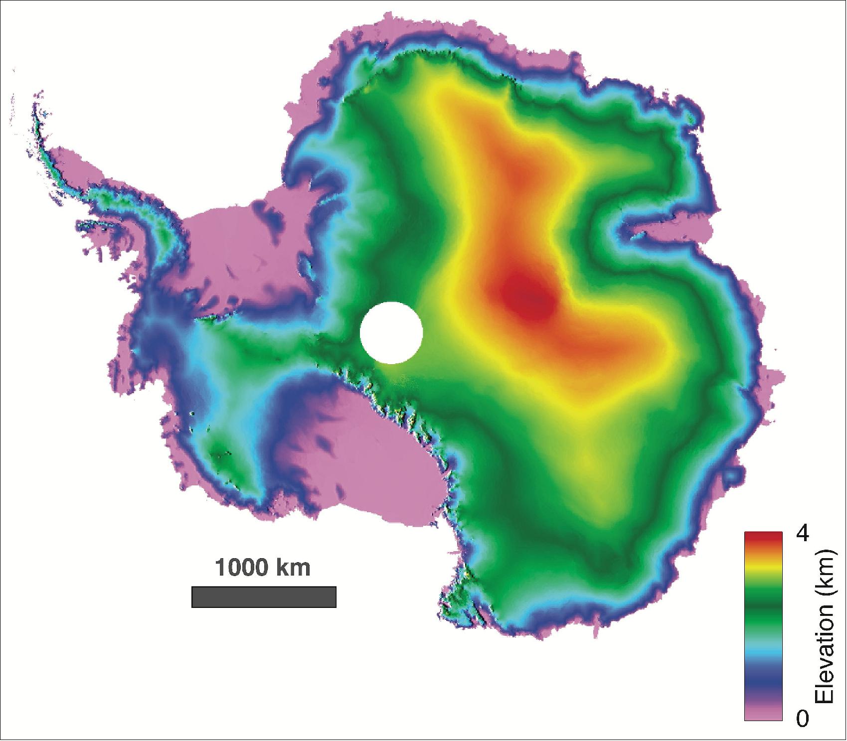
• January 23, 2019: The CryoSat users are informed that the US government shutdown currently on-going is affecting the services that are responsible for providing NOAA's input data products used in CryoSat ice and ocean processing chains. 48)
- The CryoSat L1b and L2 products with dates of validity starting on 21 December 2018 are therefore affected by this situation. As a consequence, the quality of CryoSat related geophysical corrections and derived parameters (e.g. sea ice concentration in ice products and GDP+ wet tropospheric correction in GOP) are potentially degraded.
- Users will be informed at a later stage to what extent L1b/L2 parameters are directly or indirectly impacted and once the US services return to normal.
• September 15, 2018: After eight years in orbit, the status of the satellite is very good. Funds for operating the mission have been approved until the end of December 2019 and a further extension will be proposed to extend it until end of 2021 within the current Earth Observation Envelope Program (EOEP-5). With the exception of the power subsystem, which had to be switched to its backup system in October 2013, all other satellite subsystems are on the their initial primary hardware. The on-board consumables are sufficient to operate the satellite until at least 2025. 49)
- To maintain a reference orbit with an equidistant node crossings distribution and 1 km tolerance at equator, orbit housekeeping maneuvers are required on average once a month but more often during periods of high solar activity. They are always performed to minimize impact on data return and sometimes in conjunction with Collision Avoidance Maneuvers, required to avoid space debris in collision trajectory.
The mission was originally not designed to maneuver away from space debris. However, the improvement of the space debris monitoring network and the ability to predict the threat well in advance, has allowed reconsideration of such operations and now they are part of the normal flight procedures. Since the launch, the satellite has performed thirteen Collision Avoidance Maneuvers and one of them was to avoid one piece of debris, which was at a radial distance less than 5 m from the satellite.
- The mission performance has surpassed the design specifications, delivering high quality data and providing unique contributions to several novel research and applications in Earth Science, both at global and regional scales.
- The mission has already generated data that has proven to be fundamental to the data records of sea-ice volume and ice sheet elevation changes. However, the large variety of challenges and scientific outcome emerging from the CryoSat-2 mission, identify this Earth Explorer as a classic example of a mission, scientifically intended for one domain that has successfully enlarged its portfolio of applications during its current lifetime including potential transit into an operational framework.
- Clearly, there is still much to be done. The mission will continue to determine decadal trends in ice sheets, ice caps, glaciers and sea ice mass to separate seasonal and interannual variability from long-term trends, and to robustly determine the impact of climate change on these trends. But new challenges are arising at the horizon such as the validation of the role of snow loading in the Arctic sea-ice, whose nature is now changing towards a system that is more similar to the Antarctic one.
The mission is fit to continue observations within the framework it was designed for almost two decades ago and at the same time, it is committed to taking-up new challenges counting on synergies with existing and future missions like AltiKa, ICESat-2 and Sentinels.
• May 11, 2018: Thanks to ESA's CryoSat-2 mission, a new map of Antarctica provides the most accurate 3D view ever of the continent's vast ice sheet and floating ice shelves. This latest digital elevation model, which is available for download, is a result of research published recently in The Cryosphere. The model replaces the version published in March 2017. 50)
- Tom Slater from the UK CPOM (Center for Polar Observation and Modelling) said, "Our new model has several advantages over the previous one. It covers 350,000 km2 more of the continent's surface and the resolution is twice as high, sampling the ice-sheet surface every kilometer."
- CryoSat-2's radar altimeter detects tiny variations in the height of the ice across the entire continent, including on the steeper continental margins where the vast majority of ice losses occur.
- This is about five million more than were used in the previous version, giving a snapshot of the height of the ice across 95% of the continent – a 3% increase on the 2017 version.
- Accurate knowledge of the current topography of Antarctica will allow scientists to better predict how the ice sheet will respond to a warming climate over the next decades.
- Andy Shepherd from CPOM added, "This model will also be useful to anybody wanting to know about the continent's surface, whether they are planning scientific fieldwork, or modelling the ice sheet's future behavior and potential sea level contribution."
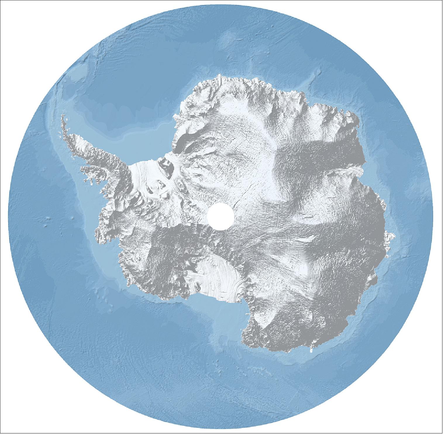
• May 2, 2018: While ESA's CryoSat-2 continues to provide clear insight into how much sea ice is being lost and how the Antarctic and Greenlandic ice sheets are changing, the mission has again surpassed its original scope by revealing exactly how mountain glaciers are also succumbing to change. Glaciers all over the globe are retreating – and for the last 15 years, glacial ice has been the main cause of sea-level rise. 51)
- Apart from Antarctica, Patagonia is home to the biggest glaciers in the southern hemisphere, but some are retreating faster than anywhere else in the world.
- This is because the weather is relatively warm and these glaciers typically terminate in fjords and lakes, exacerbating surface melting and causing them to flow faster and lose ice as icebergs at their margins.
- There is a clear need to monitor and understand glacial dynamics, not only in Patagonia but globally.
- However, with around 200,000 glaciers worldwide coupled with their remote rugged terrain, maintaining local monitoring systems is extremely difficult.
- Turning to space, satellite radar altimeters have been mapping ice loss from the large sheets for the last 25 years, but the footprint of this type of instrument is generally too coarse to monitor the smaller mountain glaciers.
- Fortunately, a new way of processing CryoSat-2 data now makes it possible to map these glaciers in fine detail.

- Noel Gourmelen from the University of Edinburgh said, "The technique of swath processing differs from conventional radar altimetry. Using CryoSat-2's novel interferometric mode, we see how the radar wave front interacts with the surface.
- "We can then extract a whole swath of elevations rather than single elevation points. This is revolutionizing the use of CryoSat-2 over complex icy terrains, yielding more detail than we ever thought possible."
- A paper published recently in Remote Sensing of Environment describes how this technique has been used to reveal complex patterns in the changing height of glaciers in Patagonia. 52)
- Luca Foresta, also from the University of Edinburgh, explained, "We've used CryoSat-2 to discover that between 2011 and 2017 there was widespread thinning, particularly in the northern part of the ice fields. For example, the Jorge Montt glacier, which flows down to the ocean, retreated 2.5 km and lost about 2.2 Gt of ice a year, and the Upsala glacier, which terminates at a lake, lost 2.68 Gt a year. In contrast, however, Pio XI, the largest glacier in South America, advanced and gained mass at a rate of about 0.67 Gt a year."
- Over the six-year period, the Patagonian ice fields overall lost mass at a rate of over 21 Gt a year, which is equivalent to adding 0.06 mm to sea level. It is also a 24% increase compared to the amount of ice lost between 2000 and 2014.
• April 3 2018: ESA's CryoSat-2 mission has revealed that, over the last seven years, Antarctica has lost an area of underwater ice the size of Greater London. This is because warm ocean water beneath the continent's floating margins is eating away at the ice attached to the seabed. 53)
- Most Antarctic glaciers flow straight into the ocean in deep submarine troughs. The place where their base leaves the seabed and begins to float is known as the grounding line. These grounding lines typically lie a kilometer or more below sea level and are inaccessible even to submersibles, so remote methods for detecting them are extremely valuable.
- A paper published today in Nature Geoscience describes how CryoSat was used to map grounding-line motion along 16 000 km of Antarctic coastline. 54)
- Research led by Hannes Konrad from the CPOM ( Center for Polar Observation and Modelling) at the UK's University of Leeds shows that between 2010 and 2017 the Southern Ocean melted 1463 km2 of underwater ice.
- The team tracked the movement of Antarctica's grounding line thanks to CryoSat-2 and has produced the first complete map showing how this submarine edge is losing its grip on the seafloor.
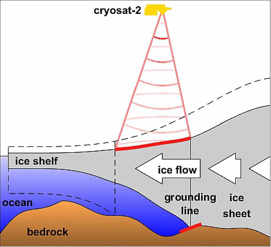
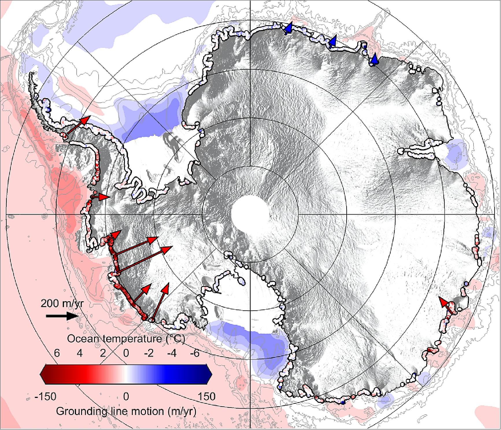
- The biggest changes are seen in West Antarctica, where more than a fifth of the ice sheet has retreated across the seafloor faster than the pace of deglaciation since the last ice age.
- Dr. Konrad said, "Our study provides clear evidence that retreat is happening across the ice sheet due to ocean melting at its base, and not just at the few spots that have been mapped before now. This retreat has had a huge impact on inland glaciers, because releasing them from the seabed removes friction, causing them to speed up and contribute to global sea-level rise."
- Although CryoSat is designed to measure changes in the ice-sheet elevation, these can be translated into horizontal motion at the grounding line using the Archimedes principle and knowledge of the glacier and seafloor geometry.
- The researchers also found some unexpected behavior (Figure 47).
- Although retreat of the Thwaites Glacier in West Antarctica has sped up, at the neighboring Pine Island Glacier – until recently one of the fastest retreating on the continent – it has halted. This suggests that the ocean melting at its base has paused.
- Dr. Konrad added, "These differences emphasize the complex nature of ice-sheet instability across the continent, and being able to detect them helps us to pinpoint areas that deserve further investigation."
- Co-author Andy Shepherd said, "We were delighted at how well CryoSat is able to detect the motion of Antarctica's grounding lines. They are impossible places to access from below so it's a fantastic illustration of the value of satellite measurements for identifying and understanding environmental change."
- ESA CryoSat mission manager Tommaso Parrinello added, "Even though CryoSat is now approaching its eighth year in orbit – more than twice its intended lifetime – it's wonderful to see that the mission is still making measurements of the highest quality and enabling new discoveries in polar science."
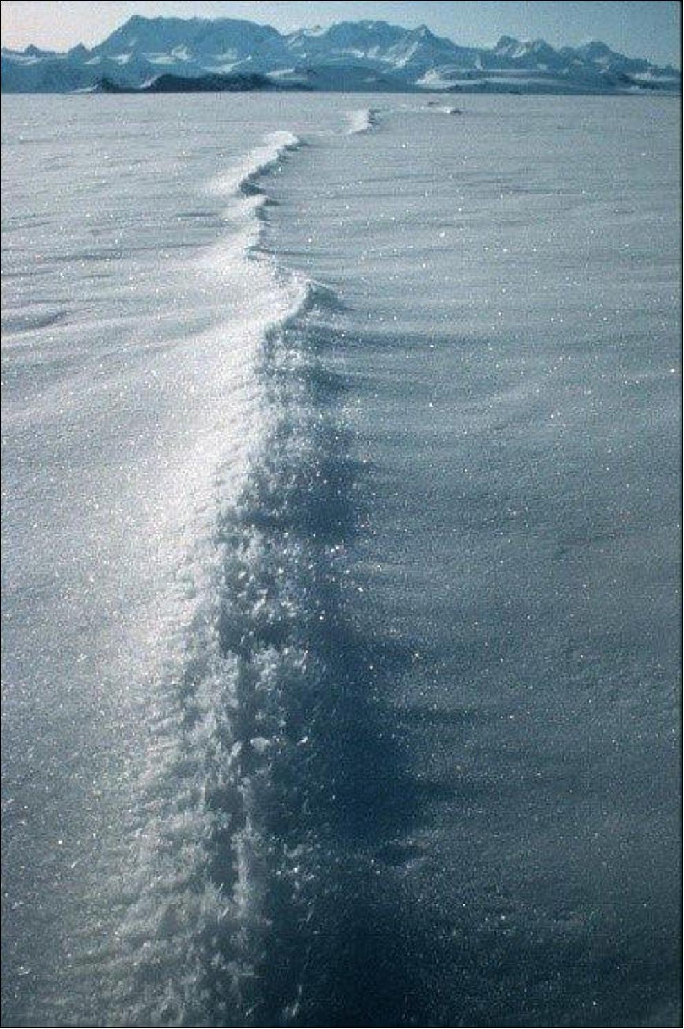
• October 11, 2017: We are all aware that Antarctica's ice shelves are thinning, but recently scientists have also discovered huge canyons cutting through the underbelly of these shelves, potentially making them even more fragile. Thanks to the CryoSat-2 and Sentinel-1 missions, new light is being shed on this hidden world. 57)
- Antarctica is surrounded by ice shelves, which are thick bands of ice that extend from the ice sheet and float on the coastal waters. They play an important role in buttressing the ice sheet on land, effectively slowing the sheet's flow as it creeps seaward.
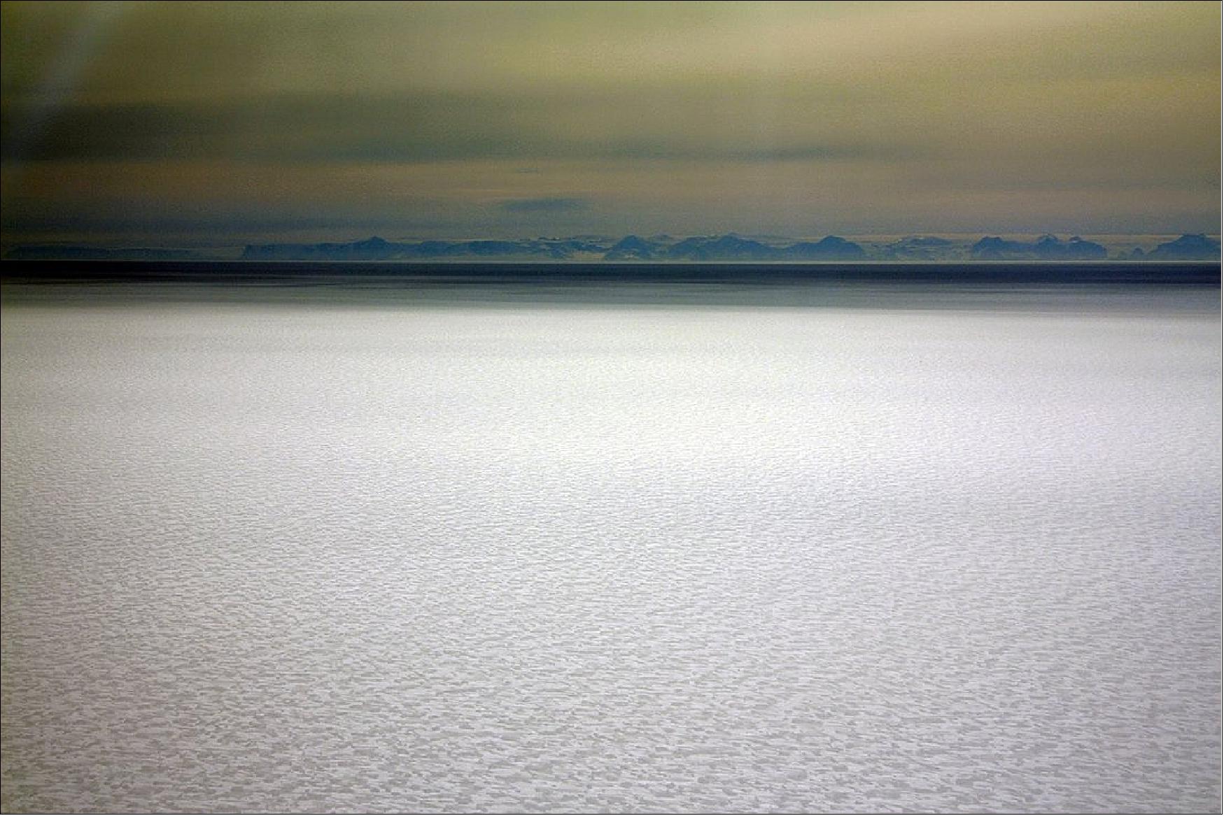
- The ice sheet that covers Antarctica is, by its very nature, dynamic and constantly on the move. Recently, however, there has been a worrying number of reports about its floating shelves thinning and even collapsing, allowing the grounded ice inland to flow faster to the ocean and add to sea-level rise.
- While scientists continue to study the changing face of Antarctica, monitor cracks in the surface of the ice that might signal the demise of a shelf and learn how these changes are affecting the biology of coastal waters, they are also aware of dramatic changes taking place below the surface, hidden from view.
- There are huge inverted canyons in the underside of ice shelves, but little is known about how they form and how they affect the stability of the ice sheet.
- One type is thought to be caused by subglacial water that drains from beneath the ice sheet and runs into the ocean. In this region, the ocean water is stratified, with the warmer water at the bottom. However, as the colder meltwater pours down into the ocean it then rises because it is less dense than the seawater – but as it rises it drags up the warm bottom water which causes the underbelly of the floating ice shelf to melt.
- Another type is thought to be caused by the way ocean water circulates under the shelf.
- Scientists have been using ESA's CryoSat-2 to study changes in the surface of the ice shelf and the Copernicus Sentinel-1 mission to study how shelves flow to learn more about what's going on hidden from view. — Their focus has been on the Dotson ice shelf in West Antarctica.
- Noel Gourmelen from the University of Edinburgh said "We have found subtle changes in both surface elevation data from CryoSat-2 and ice velocity from Sentinel-1 which shows that melting is not uniform, but has centered on a 5 km-wide channel that runs 60 km along the underside of the shelf.
- "Unlike most recent observations, we think that the channel under Dotson is eroded by warm water, about 1°C, as it circulates under the shelf, stirred clockwise and upward by Earth's rotation.
- "Revisiting older satellite data, we think that this melt pattern has been taking place for at least the entire 25 years that Earth observation satellites have been recording changes in Antarctica.
- "Over time, the melt has calved in a broad channel-like feature up to 200 m deep and 15 km across that runs the entire length of the underside of Dotson ice shelf.
- "We can see that this canyon is deepening by about 7 m a year and that the ice above is heavily crevassed.
- "Melt from Dotson ice shelf results in 40 billion tonnes of freshwater being poured into the Southern Ocean every year, and this canyon alone is responsible for the release of four billion tonnes – a significant proportion.
- "The strength of an ice shelf depends on how thick it is. Since shelves are already suffering from thinning, these deepening canyons mean that fractures are likely to develop and the grounded ice upstream will flow faster than would be the case otherwise.
- "It is the first time that we've been able to see this process in the making and we will now expand our area of interest to the shelves all around Antarctica to see how they are responding. We couldn't do this without CryoSat-2 and the European Commission's Copernicus Sentinel missions," added Dr Gourmelen.
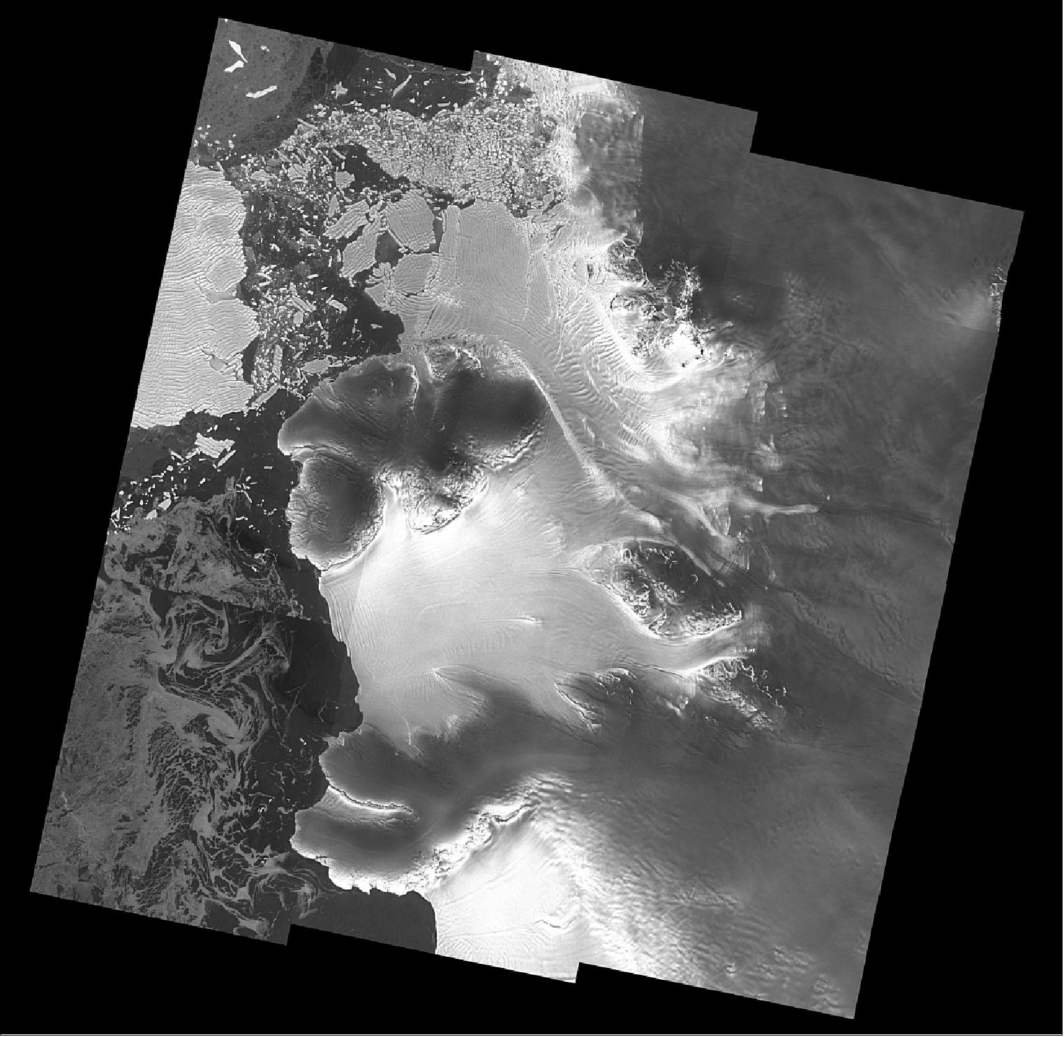
• July 5, 2017: All eyes are on Antarctica's Larsen C ice shelf as a deep crack continues to cut across the ice, leaving a huge chunk clinging on. When it eventually gives way, one of the largest icebergs on record will be set adrift. Even before the inevitable happens, ESA's CryoSat-2 mission can reveal some of the future berg's vital statistics. 58)
Monitored by the Copernicus Sentinel-1 radar pair, the crack in the ice is now around 200 km long, leaving just 5 km between the end of the fissure and the ocean. While we wait for Sentinel-1 to tell us when this 6600 km2 iceberg is spawned, CryoSat-2 can reveal what the berg's measurements will be.
This Earth Explorer satellite carries a radar altimeter to measure the height of the ice surface. In general, this information is used to work out how the thickness of sea ice and land ice is changing and, consequently, how the volume of Earth's ice is being affected by the climate.
Noel Gourmelen from the University of Edinburgh said, "Using information from CryoSat-2, we have mapped the elevation of the ice above the ocean and worked out that the eventual iceberg will be about 190 m thick and contain about 1155 km3 of ice. "We have also estimated that the depth below sea level could be as much as 210 m."
Icebergs calve from Antarctica all the time, but because this one is particularly large its path across the ocean needs to be monitored as it could pose a hazard to maritime traffic.
Again, Sentinel-1 and CryoSat-2 will play an important role in tracking the berg and keeping an eye on how it changes. Dr Gourmelen added, "We will continue to use CryoSat-2 to monitor how the berg changes as it drifts away from the ice shelf."
A berg, similar in size, drifted around the Brunt ice shelf in December 2015, causing alarm for those stationed at the Halley research base, which sits on the floating section of the shelf.
Anna Hogg from the University of Leeds said, "Measurements from CryoSat showed that the Brunt berg was around 390 m, so too thick to come close to ‘shore' since the sea is shallow here.
"As for this new Larsen C berg, we are not sure what will happen. It could, in fact, even calve in pieces or break up shortly after. Whole or in pieces, ocean currents could drag it north, even as far as the Falkland Islands. If so it could pose a hazard for ships in Drake Passage. What is certain, though, is that we shall continue to use CryoSat to keep a check on its progress."
ESA's Mark Drinkwater added, "Our historical effort to track large icebergs shows that those from the western Weddell Sea find their way out into the Antarctic Circumpolar Current or into the South Atlantic. It seems that only bergs from the Ross ice shelf stay in the westward coastal current and come close to Brunt ice shelf."
The main purpose of CryoSat-2 is to give us information to understand how ice is changing to improve our understanding of Earth. The value of having satellites built to deliver for science and missions like Sentinel-1, which are built to deliver for everyday applications, is enormous.
In this case, the Copernicus Sentinel-1 mission and the ESA Earth Explorer CryoSat-2 mission complement each other, giving us a powerful tool to monitor changing ice sheets.
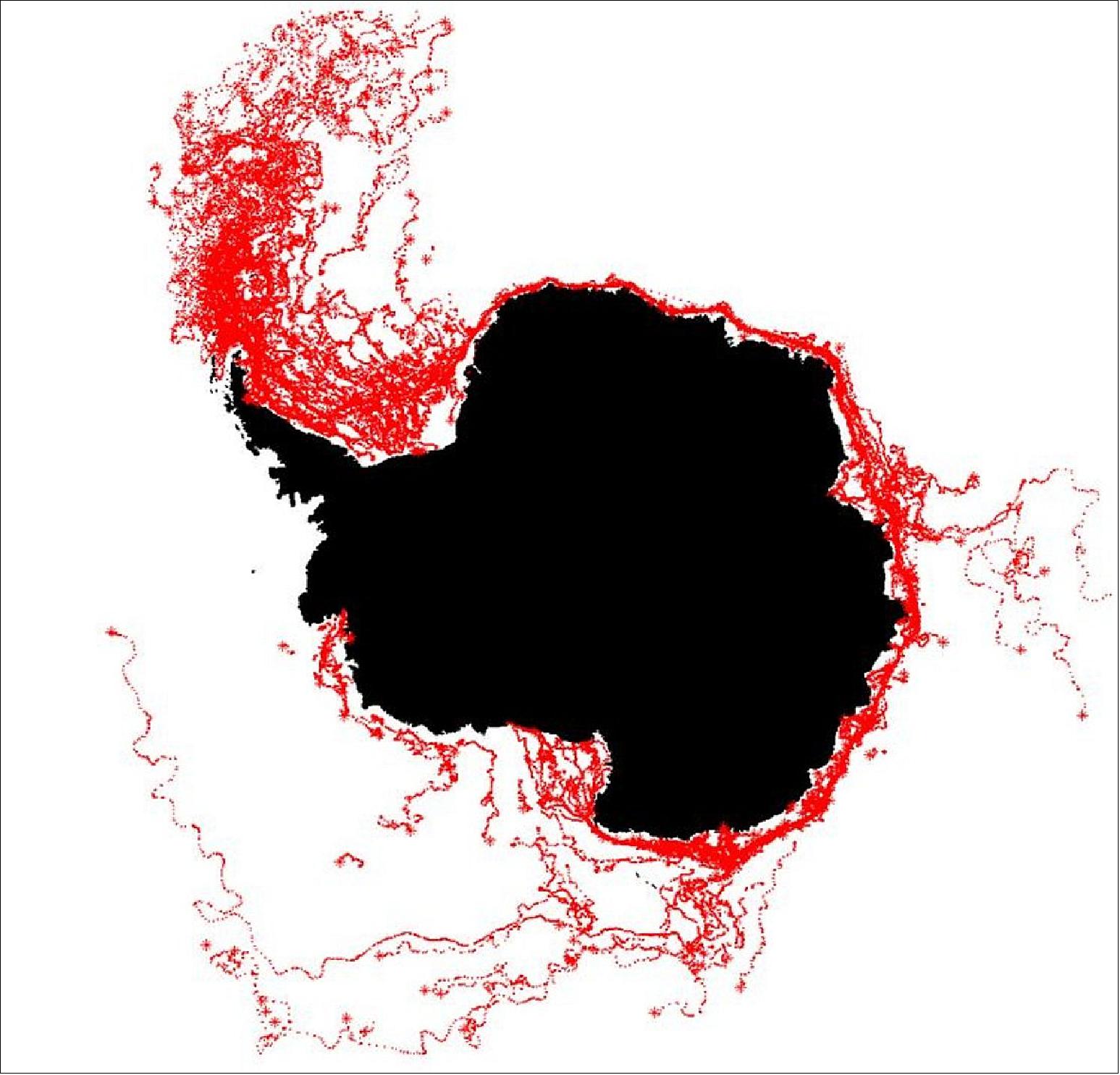
• March 24, 2017: Around 250 million measurements taken by ESA's CryoSat-2 over the last six years have been used to create a unique 3D view of Antarctica, offering a snapshot of the undulating surface of this vast ice sheet. 60)
- CryoSat's radar altimeter detects tiny variations in the height of the ice across the entire continent, including on the steeper continental margins where the vast majority of ice losses occur. Importantly, the satellite's orbit takes it to latitudes within 200 km of the north and south poles – closer than other Earth observation satellites. Naturally, the mission is also used to map changes in the thickness of ice floating in the polar oceans, which is particularly important for the Arctic.
- The new ‘digital elevation model' of Figure 52 was revealed at this week's gathering of CryoSat scientists in Banff, Canada. Tom Slater, researcher at the UK CPOM (Centre for Polar Observation and Modelling), said, "We used around 250 million measurements taken by CryoSat between 2010 and 2016 to create the most comprehensive picture of Antarctic ice elevation currently available." It offers wide range of applications – showing the surface of Antarctica in such detail means it can be used in anything from planning fieldwork to modelling the ice sheet.
- It also allows scientists to distinguish between changes in topography and ice motion when working with other satellite measurements, such as those used to calculate the balance between how much the ice sheet is gaining by accumulating snow and losing through melting and creating icebergs.
- The model will soon be freely available via the CPOM portal, which already provides information on sea-ice volume and thickness, ice velocity and, shortly, ice sheets. In the meantime, however, the model can be downloaded here.
- CPOM Director Andrew Shepherd added, "We want the digital elevation model to be accessible to anyone who uses ice-sheet surface topography measurements in their work. This should benefit not only studies of the Antarctic ice sheet, but also projections of future sea-level rise."
- ESA's CryoSat mission manager, Tommaso Parrinello, said, "We are hearing some great results from our mission at the meeting here in Banff.
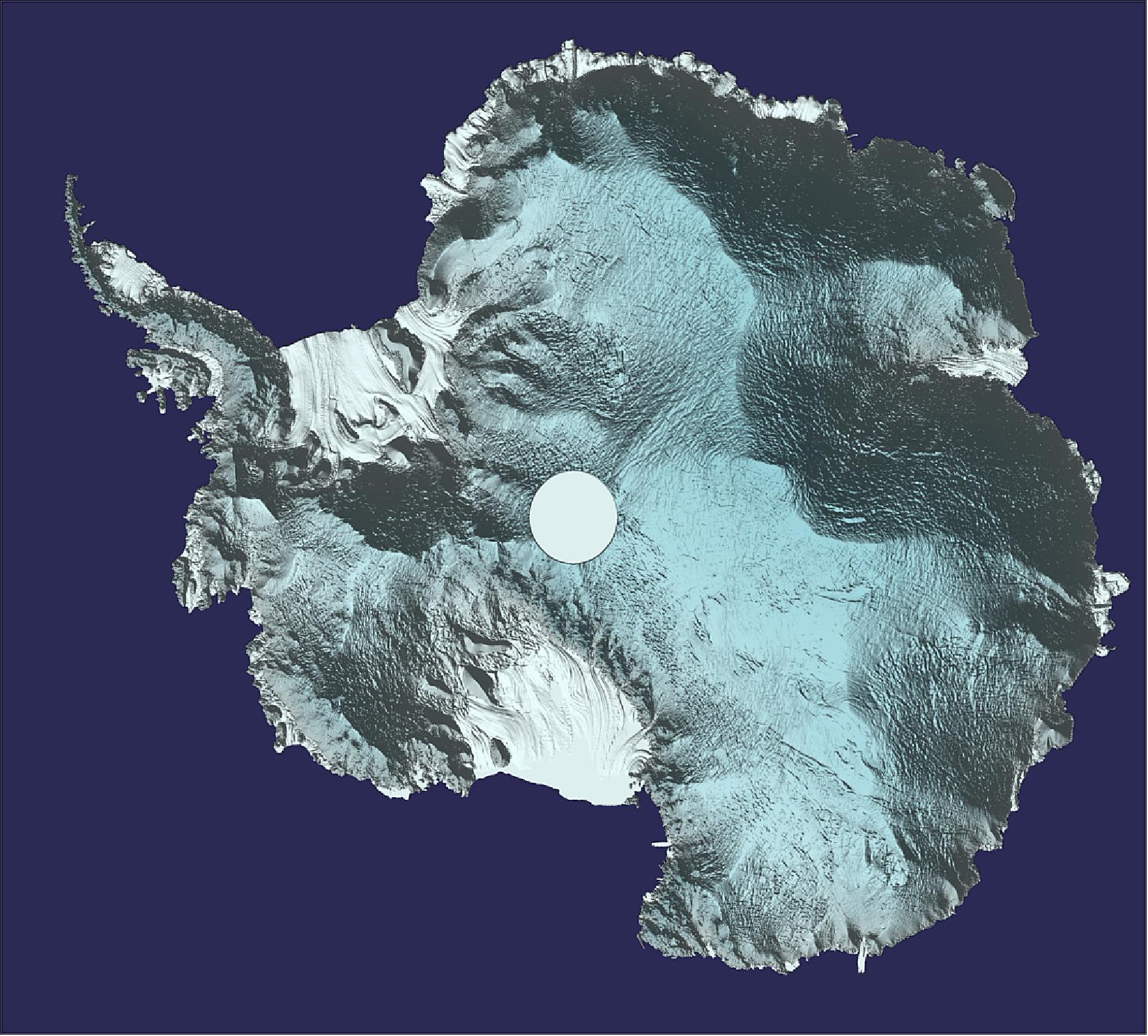
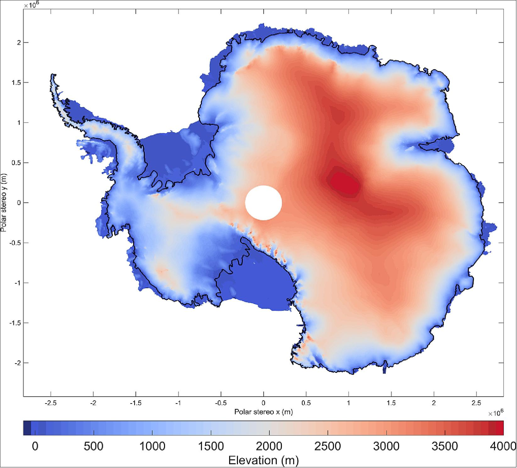
• March 20, 2017: After the relative quiet of the long dark winter months, the Arctic will be a tad busier over the coming weeks as numerous researchers descend on this harsh, yet fragile environment. Their aim is not to disturb its beauty, but to join forces in an all-out effort to measure ice on land and sea. 61)
- Environmental changes in the Arctic are no longer only of interest to scientists. The need to understand and respond to dwindling polar ice is being given increasing importance at global climate discussions and vital for adopting strategies to mitigate and to adapt to change.
- Unequivocal evidence of changing polar ice comes largely from satellites. Since it was launched in 2010, ESA's CryoSat-2, orbiting at an altitude of 700 km, has been measuring the height of the ice, both of that floating in the polar oceans and of the vast ice sheets covering Greenland and Antarctica. This provides essential information on how the thickness is changing and, in turn, how the volume of ice is changing.
- Over the last seven years, there have been several expeditions to the Arctic that involve taking measurements with a suite of sensors on aircraft and readings taken by hand actually on the ice to compare with those of CryoSat-2. By doing all this, scientists can ensure that ice-thickness maps created from satellite data are correct.
- This week sees the beginning of one of the largest Arctic expedition ever undertaken by ESA, the CryoVEx (CryoSat Validation Experiment) campaign. "We have scientists from around 10 agencies and institutes from all over the world converging in the Arctic," explained Malcolm Davidson, head of ESA Earth observation campaigns. "We are pooling resources with other agencies such as NASA and other institutes to make our campaign a huge collaborative international effort."
- Arne Olesen from DTU (Technical University of Denmark) added, "And, with so many people prepared to work for weeks in the most remote places on the planet and put up with the extreme cold and hazardous conditions, it just reflects how passionate and dedicated everyone is about polar science and getting the best data possible."
- There is another purpose: to prepare for future satellite missions similar to CryoSat-2, but with even better measurement capabilities. Malcolm Davidson continued, "Our understanding of changing ice has improved enormously thanks to CryoSat-2, but we must prepare for the future now and test new types of sensors that may be able to give us even better information.
- "So, while we are out in the Arctic, we will be testing a new concept that involves a radar altimeter (Figure 54) that works with two different wavelengths instead of only one like on CryoSat-2. It's always very exciting to be at the forefront of new technology. It is essential that we put in the groundwork to make sure a new concept will work – and, in this case, it means getting very cold and even the prospect of facing the occasional polar bear!"
- While the expedition gets underway, CryoSat-2 is also the focus of a conference in Alberta in Canada this week. Here, scientists have come together to discuss the latest results emerging from the mission.
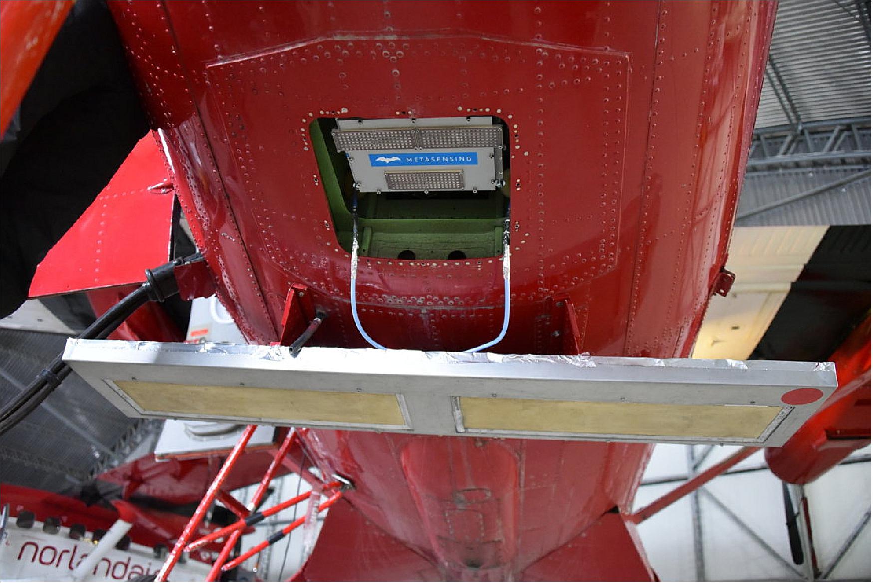
• February 8, 2017: A novel way of using ESA's CryoSat-2 mission has revealed how lakes beneath the Thwaites Glacier drained into the Amundsen Sea – potentially the largest such outflow ever reported in this region of West Antarctica. This new information is helping scientists understand more about what's going on deep below the surface of the ice and what affects how fast the glaciers flow towards the ocean. Thwaites and its neighboring Pine Island Glacier are the fastest-receding glaciers on the Western Antarctic Ice Sheet. 63) 64)
- Although this huge sheet is some 2 km thick in places, much of its floor is well below sea level. This makes it particularly vulnerable to change, especially where the warmer ocean waters meet the underside of the floating terminus of the glacier.
- Understanding the movements of these glaciers is critical for predicting how the ice sheet may behave in the future and how it may affect sea level.
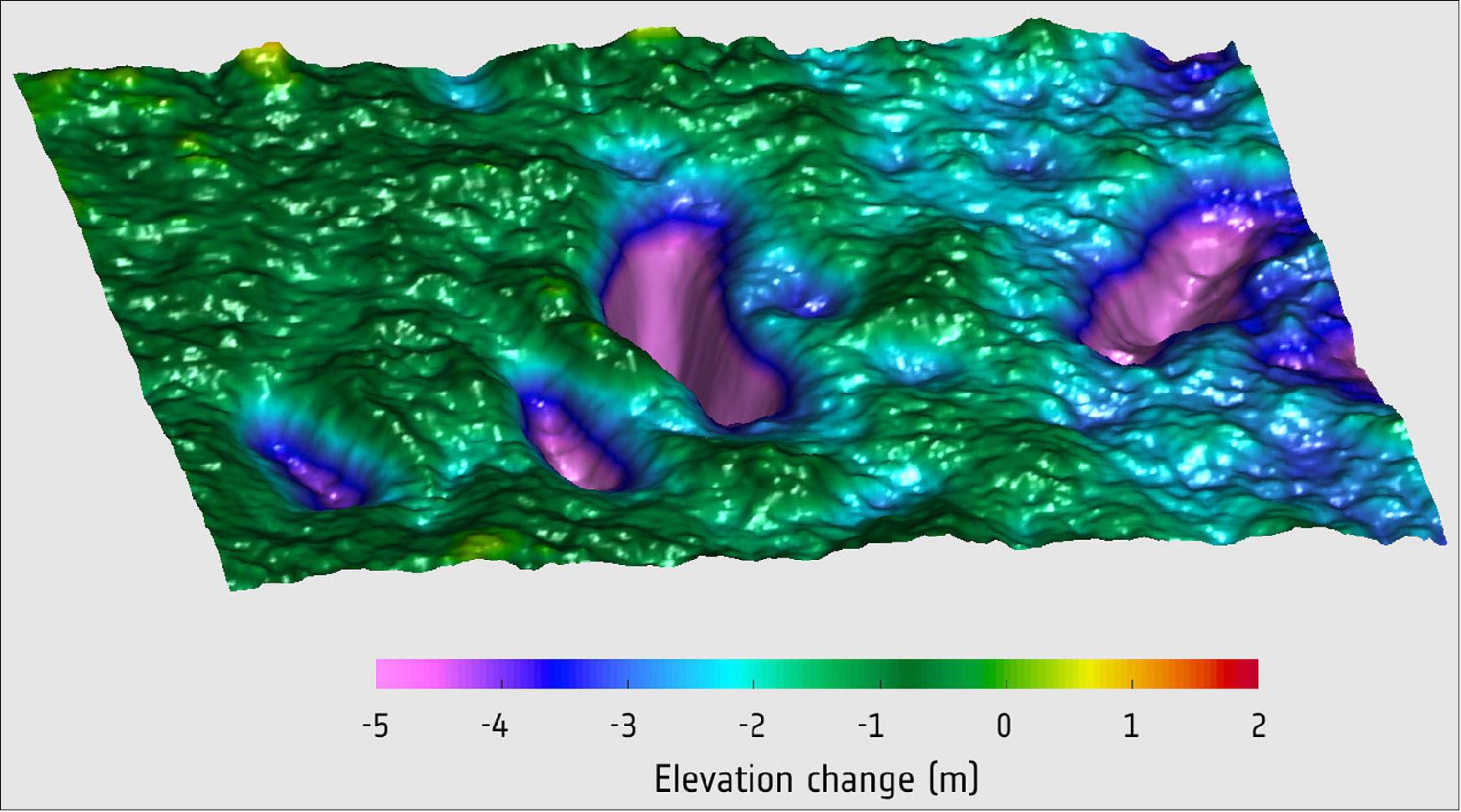
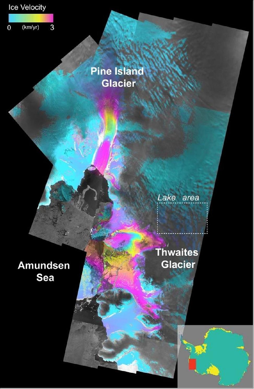
- Lakes have been found under glaciers in many parts of Antarctica and are, indeed, commonly associated with fast-flowing glaciers. However, this is the first time they have been found and observed draining into the Amundsen Sea. In addition, this emptying is thought to happen only every 20–80 years.
- Water below the ice sheet plays an important role in how quickly glaciers flow towards the sea, thought to be because a layer of meltwater reduces friction between the ice and the bedrock.
- In addition, when channels form under the ice they lubricate the glacier bed.
- Benjamin Smith from the University of Washington (Seattle, WA, USA) and lead author of the paper said, "This is first time we've been able to monitor both elevation changes and ice speed in this kind of detail over such a large area. Without a satellite like CryoSat, we would have probably have missed the lake draining and we would have had to guess how the lake drainage might have affected the ice speed. Together, they tell us about how water moving at the glacier bed affects ice speed, and what processes we need to understand so that we are better equipped to predict the future of Thwaites."
- Noel Gourmelen from the University of Edinburgh explained, "Repeat observations from CryoSat-2 over Thwaites revealed that the surface of the ice subsided by several meters as water drained away from the four lakes under the ice. The lakes totalled an area of about 700 km2. On average, Thwaites carries about 135 km3 of ice to the sea every year, but drainage from these lakes released an extra 3.5 km3 of freshwater. In addition, the speed of the glacier increased by about 10% and would have contributed to a discharge of around 150 km3 a year between 2013 and 2014."
- Drainage is estimated to have peaked at about 240 m3 per second, possibly the largest outflow of meltwater ever reported from subglacial lakes in this region. This peak rate is about four times faster than the River Thames in England discharges to the North Sea each year.
- Before this discovery, scientists had thought that this part of the ice sheet did not store water in lakes beneath the surface for very long because abrupt drainage had not been seen before in the area.
- Mark Drinkwater, head of ESA's Earth observation mission science, said, "Previous studies have investigated if CryoSat-2 could be used for monitoring small vertical displacements associated with these events. The main issue has been the limited coverage of standard altimeter measurements. But thanks to new processing techniques, the capability of using CryoSat-2 to both discover and monitor Antarctic subglacial lakes has vastly increased."
- Tommaso Parrinello, ESA's CryoSat-2 mission manager, added, "CryoSat again is proving what a versatile satellite it is. Now we also have the Copernicus Sentinel-1, with both providing powerful tools for developing further understanding of the relationship between lake drainage and ice dynamics in Antarctica."
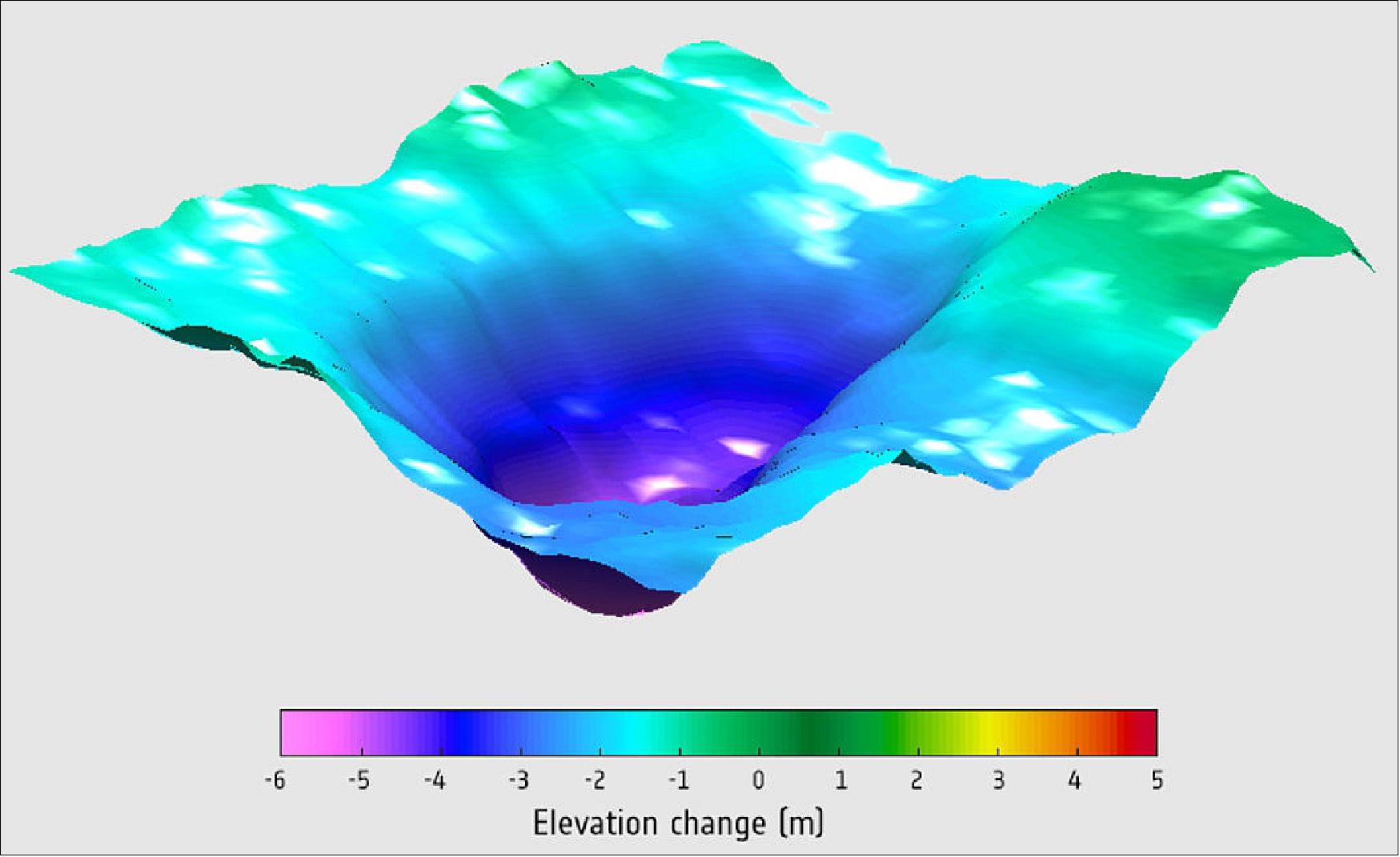
• December 16, 2016: Although not designed to deliver information on ice, ESA's Earth Explorer SMOS satellite can detect thin sea-ice. Since its cousin, CryoSat-2, is better at measuring thicker ice scientists have found a way of using these missions together to yield an even clearer picture of the changing Arctic. 66)
- Carrying a radiometer, SMOS was designed capture images of brightness temperature. While these images can be turned into information on soil moisture and ocean salinity to improve our understanding of the water cycle, it turns out that these data can also be used to measure sea ice.
- In contrast, CryoSat-2 carries a radar altimeter that measures freeboard of sea ice, which is the distance between the waterline and the top of the ice.
- This is being used to work out how the thickness of sea ice is changing and, in addition, how the volume of Earth's ice is being affected by the climate.
- Despite the two missions being very different, scientists from the University of Hamburg and the AWI (Alfred Wegener Institute) in Bremerhaven, Germany, who are involved in both Earth Explorer missions, have found a way of combining data from both satellites to gain a more complete picture of changes in the thickness of ice floating in Arctic waters. — While the accuracy of measurements from CryoSat-2 increases with increasing ice thickness, SMOS data are more accurate when the sea ice is relatively thin, less than about a meter.

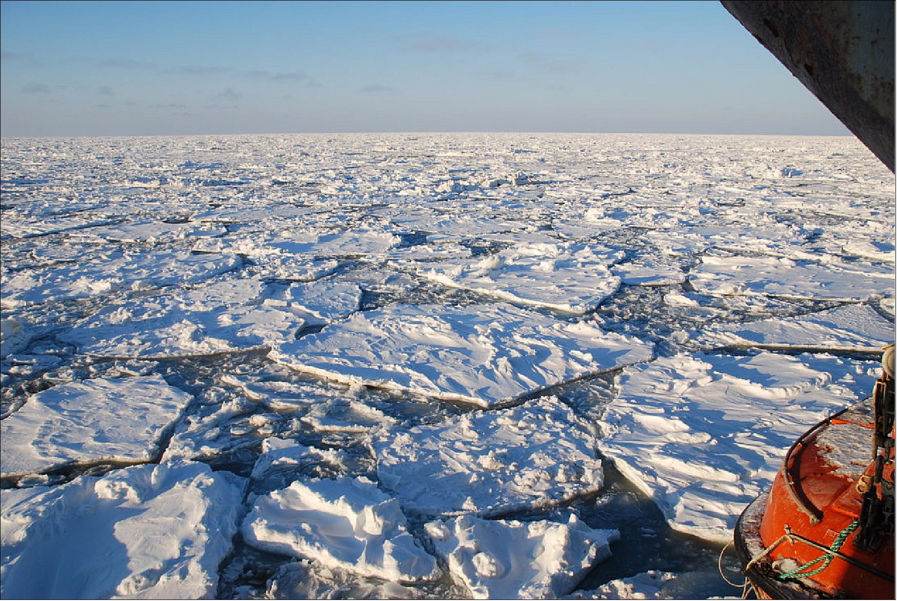
- CryoSat measurements yield high-spatial resolution information and cover the Arctic every month. While SMOS offers daily images, they are a much coarser resolution than those of CryoSat-2. Robert Ricker from AWI said, "By combining ice-thickness estimates from CryoSat-2 and SMOS, we obtain a more accurate and comprehensive view on the actual state of Arctic sea ice. Users need timely information across the entire Arctic and we can meet their needs by combing information from these two different, but complementary satellite missions."
- The University of Hamburg is already using SMOS to provide daily maps of Arctic sea-ice thickness during the winter. These maps are produced within 24 hours of the measurements being taken in space. SMOS is also helping to improve the accuracy of sea-ice forecasts, which could help marine traffic operators to determine the safest and most economic routes through waters such as the Northwest Passage and the Northern Sea Route as the ice becomes thinner owing to climate change.
- In addition, both missions' archived data have been merged to generate information on thin sea-ice going back to 2010.
- This will make an important contribution to studies into the fragile component of the Earth system and help to understand annual variations and climate change. Lars Kaleschke, from the University of Hamburg, emphasized, "It is good see how information from two different types of measurements can be combined into one product to advance science and improve operational applications. It has now been demonstrated that using ice thickness information from SMOS improves the model computations and forecasts. It will be interesting to see how ocean current and air temperature models will benefit from a better understanding of the sea-ice fields."
• November 30, 2016: ESA's CryoSat-2 satellite has found that the Arctic has one of the lowest volumes of sea ice of any November, matching record lows in 2011 and 2012. Early winter growth of ice in the Arctic has been about 10% lower than usual. - CryoSat carries a radar altimeter that can measure the surface height variation of ice in fine detail, allowing scientists to record changes in its volume with unprecedented accuracy. These observations are vital for tracking climate change and are an essential resource for maritime operators who increasingly navigate the icy waters of Earth's polar regions. 67)
- The US NSIDC (National Snow and Ice Data Center) reported that the area of the Arctic covered by sea ice fell to 4.1 million km2 in September this year – slightly less than the sea-ice extent in September 2011. - But CryoSat-2 shows that the ice was thicker at the end of summer than in most other years, at 116 cm on average. This means there was substantially more ice this year than in 2011.
- Thicker ice can occur if melting is lower, or if snowfall or ice compaction is higher. However, the Arctic usually gains about 161 km3 of ice per day in November, but this year's growth has been about 10% lower, at 139 km3 per day, with a total ice volume estimated to have accumulated to 10,500 km3 by the end of the month.
- This would essentially tie with conditions in the Novembers of 2011, when levels were at their lowest on record for this time of the year. Although sea ice in the central Arctic is currently thicker than it was in 2011, there is far less ice in more southerly regions such as the Beaufort, East Siberian and Kara Seas.
- "Because CryoSat can measure Arctic sea ice thickness in autumn, it gives us a much clearer picture of how it has fared during summer," said Rachel Tilling, at the UK's CPOM (Center for Polar Observation and Modelling), who came to these conclusions. "Although sea ice usually grows rapidly after the minimum extent each September, this year's growth has been far slower than we'd expect – probably because this winter has been warmer than usual in the Arctic."
- As demand for information on Arctic conditions increases, CryoSat-2 has become an essential source of information for polar stakeholders, ranging from ice forecasting services to scientists studying the effects of climate change. "In its short, six years of life, we have learnt more about Arctic sea ice from CryoSat-2 than from any other satellite mission," commented CPOM Director and principal scientific advisor to the CryoSat mission, Professor Andrew Shepherd. "To understand the role that sea ice plays in the climate system, and the restrictions it places on maritime operations, we must ensure that its measurements are continued into the future."
- CPOM plans to release a complete assessment of 2016 sea ice conditions in the coming weeks.
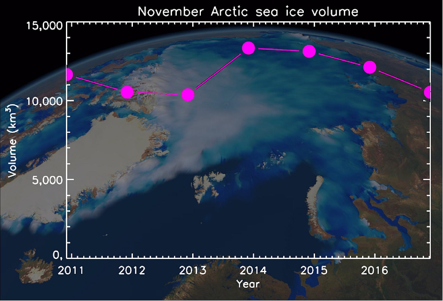
• July 26, 2016: Trying to measure sea levels around rugged coastlines is not always an easy task. ESA’s CryoSat-2 satellite is making a difference with its radar altimeter. Sea level is a very sensitive indicator of climate change, reflecting components of the climate system such as heat, glaciers and the melting of ice-sheets. Precisely monitoring changes in the average level of oceans is vitally important for understanding not only climate but also the social and economic consequences of any rise in sea level, especially in coastal zones. Previous radar altimeters have been aimed at measuring oceans and land, but CryoSat’s is the first sensor of its kind designed for ice, and able to map sea levels with unprecedented accuracy. 68)
- Scientists from the Norwegian University of Life Sciences also discovered that CryoSat had the potential to map sea level closer to the coast. Using satellite altimeters in coastal zones is notoriously difficult. Norway boasts the world’s second longest coastline of some 100,000 km, comprising many islands, steep mountains and deep, narrow fjords. The rugged coastline means that other altimeters produce confused readings close to the coast, showing differences of 10 cm or more. By contrast, CryoSat’s results compare favorably with the Stavanger tide gauge in southwestern Norway, provided by the Norwegian Mapping Authority.
- While classical altimetry offers a few tens of observations over a five-year period, more or less near a tide gauge, some 7000 measurements very close to the gauge are obtainable with CryoSat-2. The result is a better affinity with the Stavanger data, to within 7 cm for CryoSat-2, contrasting with the 10–15 cm for classical altimetry. This demonstrates the superior accuracy of CryoSat-2 in the coastal zone, where the regional impact of sea level rise is more important for humans.
- “Conventional altimeters on satellites like Envisat and Jason-3 typically have 10–30 times larger footprint than the new altimeters on CryoSat and Sentinel-3,” comments Ole Baltazar Andersen, senior scientist at the National Space Institute and DTU Space of Denmark. “Hence, the radar pulse used to measure the sea-surface height is more frequently disturbed in the coastal zone. Therefore, you have to go further from the coast to obtain accurate observations with conventional altimeters. “Consequently, you are not measuring the sea-surface height right at the coast, as we now can with CryoSat and Sentinel-3.” CryoSat-2 also gives favorable results along the remaining Norwegian coast. In comparison with the Kabelvåg tide gauge in the Lofoten area in northern Norway, differences as low as 5.4 cm were obtained. There are now great expectations from the more recent Sentinel-3 mission, which carries a similar altimeter.
• July 21, 2016: After six years in orbit, the status of the satellite remains very good. Funds for operating the mission have been approved until the end of February 2017 and a further extension is foreseen into the next phase of the EOEP-5 (Earth Observation Envelope Program). With the exception of the power subsystem, which switched to its redundant side in October 2013, all other subsystems on the satellite remain in their prime. The onboard consumables are sufficient to operate the satellite until 2025. Recently, the onboard startracker software has been upgraded to improve robustness and performance ready for the next mission extension phase. 69)
- Since launch, the CryoSat ground segment has evolved significantly and has included new products in response to requirements coming from various scientific communities, mainly from areas such as oceanography, marine gravity and hydrology. Two major versions of CryoSat product portfolio have been released to users since launch and a new one is expected by the end of 2017. - The number of CryoSat users has more than tripled during its first six years in orbit, confirming the high level of interest of the worldwide scientific community in this mission.
• April 21, 2016: Sea ice physicists from the AWI (Alfred Wegener Institute) / Helmholtz Center for Polar and Marine Research (Bremerhaven, Germany), are anticipating that the sea ice cover in the Arctic Ocean this summer may shrink to the record low of 2012. The scientists made this projection after evaluating current satellite data about the thickness of the ice cover. The data show that the arctic sea ice was already extraordinarily thin in the summer of 2015. Comparably little new ice formed during the past winter. Today Marcel Nicolaus, expert on sea ice, has presented these findings at a press conference during the annual General Assembly of the European Geosciences Union in Vienna. 70)
- Predicting the summer extent of the arctic sea ice several months in advance is one of the great challenges facing contemporary polar research. The reason: until the end of the melting season the fate of the ice is ultimately determined by the wind conditions and air and water temperatures during the summer months. Foundations are laid during the preceding winter, however. This spring, they are as disheartening as they were in the negative record year of 2012. Back then, the sea ice surface of the Arctic shrunk to a record low of 3.4 million km2.
- “In many regions of the Arctic, new ice only formed very slowly due to the particularly warm winter. If we compare the ice thickness map of the previous winter with that of 2012, we can see that the current ice conditions are similar to those of the spring of 2012 – in some places, the ice is even thinner,” Marcel Nicolaus, sea ice physicist at AWI, said today at a press conference during the EGU (European Geosciences Union) General Assembly in Vienna. 71)
- Together with his AWI colleague Stefan Hendricks, they evaluated the sea ice thickness measurements taken over the past five winters by the CryoSat-2 satellite for their sea ice projection. Seven autonomous snow buoys, which the AWI researchers had placed on floes last autumn, supplied additional important clues. In addition to the thickness of the snow cover on top of the sea ice, the buoys also measure the air temperature and air pressure. A comparison of their temperature data with the AWI long-term measurements taken on Spitsbergen, has shown that the temperature in the central Arctic in February 2016 exceeded average temperatures by up to 8ºC.
Buoy data show: the sea ice did not melt during the winter, but it grew only slowly.
- Contrary to a report published by US researchers, this warmth did not result in the thinning of the sea ice cover in some regions over the course of the winter. “According to our buoy data from the spring, the warm winter air was not sufficient to melt the layer of snow covering the sea ice, let alone the ice itself,” Marcel Nicolaus explains. During the past winter, the growth of the arctic sea ice was significantly slower than the scientists had expected.
- In previously ice-rich areas such as the Beaufort Gyre off the Alaskan coast or the region south of Spitsbergen, the sea ice is considerably thinner now than it normally is during the spring. “While the landfast ice north of Alaska usually has a thickness of 1.5 meters, our US colleagues are currently reporting measurements of less than one meter. Such thin ice will not survive the summer sun for long,” Stefan Hendricks, AWI sea ice physicist, explained.
Large amounts of thick pack ice will be carried away by Arctic sea currents before the autumn.
- Examining the CryoSat-2 sea ice thickness map for this spring, Stefan Hendricks further explained: “The Transpolar Drift Stream, a well-known current in the Arctic Ocean, will be carrying the majority of the thick, perennial ice currently located off the northern coasts of Greenland and Canada through the Fram Strait to the North Atlantic. These thick floes will then be followed by thin ice, which melts faster in the summer. Everything suggests that the overall volume of the arctic sea ice will be decreasing considerably over the course of the coming summer. If the weather conditions turn out to be unfavorable, we might even be facing a new record low,” Stefan Hendricks said.
- According to the AWI scientists, the extent of the ice loss will be great enough to undo all growth recorded over the relatively cold winters of 2013 and 2014. AWI researchers observed a considerable decrease in the thickness of the sea ice as early as the late summer of 2015, even though the overall ice covered area of the September minimum ultimately exceeded the record low of 2012 by approximately 1 million km2. The unusually warm winter has thus contributed to the likely continuation of the dramatic decline of the Arctic sea ice throughout 2016.
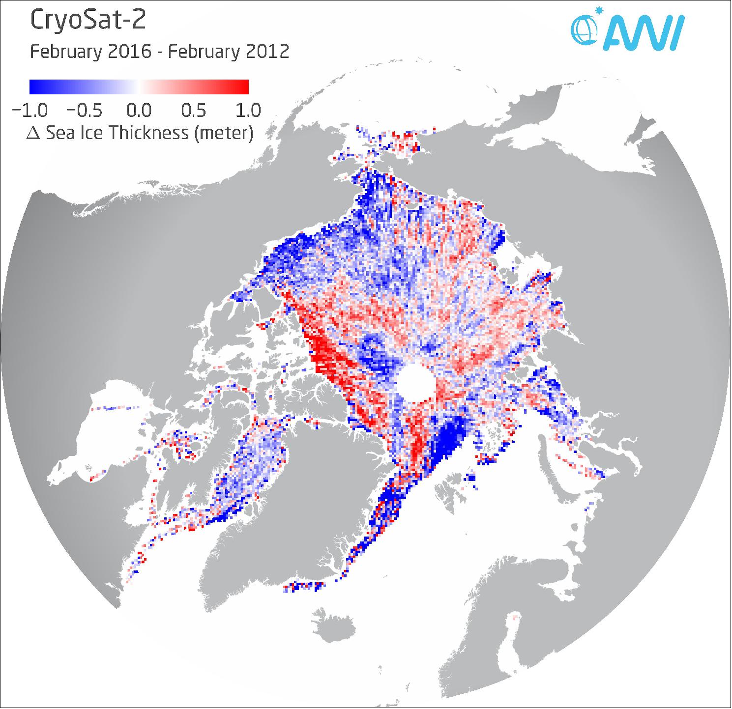
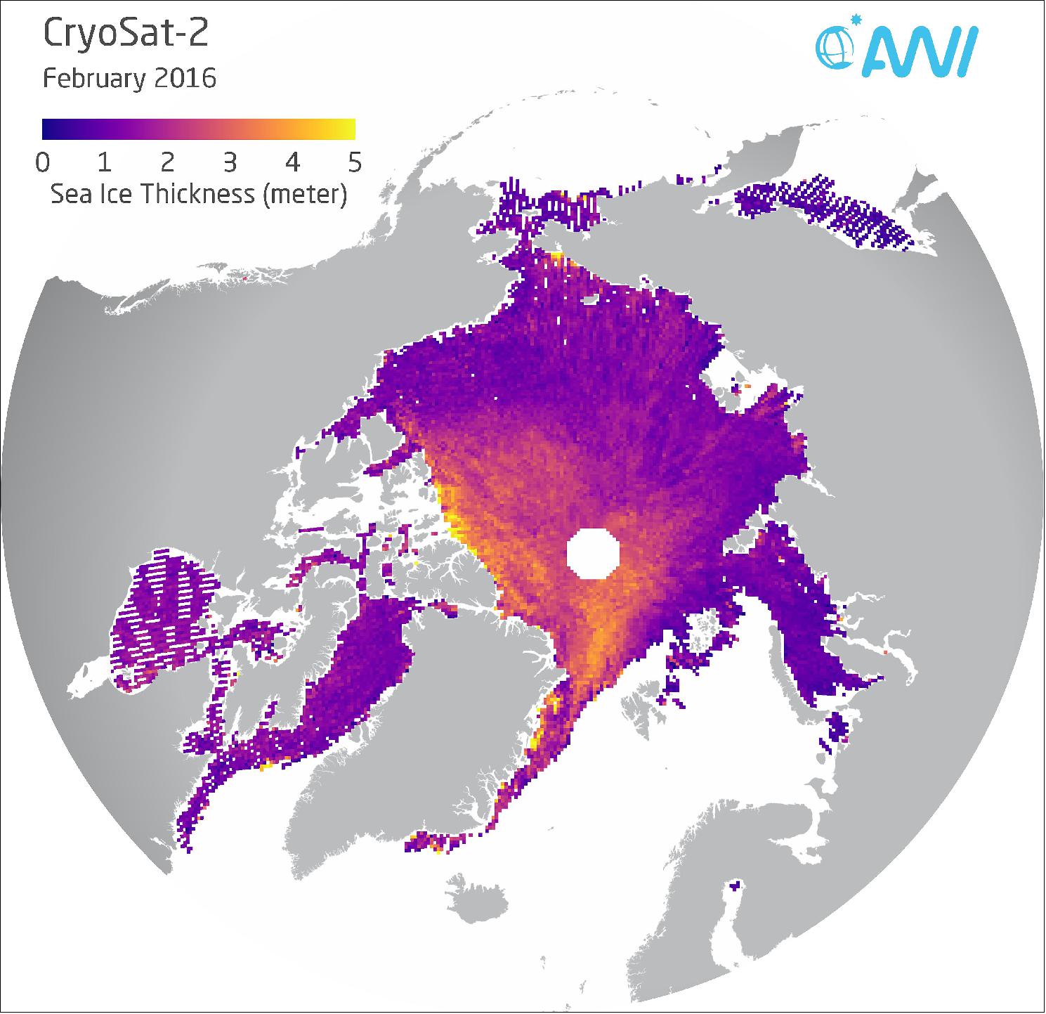
• March 2016: Urgent call for a follow-up mission. A group of 179 researchers is concerned the ageing CryoSat-2 mission could die in orbit at any time. They have urged the EC (European Commission) and ESA (European Space Agency) to start planning a replacement. "The mission is now central to international efforts to monitor the state of the cryosphere," they write in a letter to top officials at the EC and ESA. 72)
- CryoSat-2 was launched in 2010 on what was initially supposed to be just a one-off, three-and-half-year observation of marine and land ice - to get a snapshot of any gains and losses. But the performance of the spacecraft's mapping instrument SIRAL ( SAR Interferometer Radar Altimeter) - has exceeded all expectations, and made for some compelling data sets. The satellite has delivered the first complete assessment of Arctic sea-ice thickness and volume, as well as the most precise measurements yet of the volume and mass of the great ice sheets covering Antarctica and Greenland.
- "Over recent years, the ESA CryoSat-2 satellite has significantly improved our understanding of how polar ice sheets - in particular, the WAIS (West Antarctic Ice Sheet) - are changing and contributing to current global sea-level rise," said letter signatory Prof David Vaughan, the director of science at the British Antarctic Survey. "Many of the recent improvements in the models we use to predict the future of the WAIS were driven by the requirement to accurately simulate CryoSat's observations. So maintaining the record of ice-sheet change in future decades will be vital if we are to achieve the most rapid possible improvements in future projections of sea-level rise," he told BBC News.
- How long CryoSat-2 can keep working is anyone's guess. It has enough fuel to sustain itself into the early 2020s but component failure in the harsh environment of its orbit, 720 km above the Earth, is an ever-present risk.
- If there is to be a CryoSat-3, it will not come directly out of the ESA stable. The agency's job is to develop new technologies; its remit does not extend to funding ongoing, repeat missions. This means a successor would fit better within the Copernicus series of satellites - known as the Sentinels - which are currently being rolled out by the European Commission, paid for by EU member states; ESA participates only as the technical advisor.
- One of these new platforms, Sentinel-3, can do some work in polar regions: it has a radar altimeter to sense ice surfaces, too. But the spacecraft's orbit does not reach the same heights, meaning its data contains a 1,860 km wide "hole" at northernmost and southernmost latitudes. This makes it blind to most Arctic sea-ice, for example. Additionally, Sentinel-3's radar does not operate in a so-called interferometric mode. This is the capability that allows CryoSat to measure the slopes and ridges at the edges of the ice sheets, where losses in Antarctica and Greenland have been most pronounced.
- "The Copernicus program is a phenomenal achievement for Europe and Sentinel-3 will be doing vital work, especially over the oceans, but we'd really like to see Copernicus incorporate a proper polar Sentinel," said Prof Andy Shepherd, the principal scientific advisor to the CryoSat mission.
- The scientists are hoping for a swift process with a positive outcome. They want to avoid the gap in observations that would arise if CryoSat-2 fails and a successor is not ready. "A continuation assures a consistency in the estimates of the contribution of ice sheets to sea level change using altimetry," explained Prof Angelika Humbert from the Alfred Wegener Institute for Polar and Marine Research, Germany. "The highly sophisticated processing scheme and the error estimates are established already. In short, we know the sensor well; we've already got quite far with whatever we can squeeze out from its signals and the most benefit, with most efficiency, would come from continuing the mission."
• December 11, 2015: The satellite age has revolutionized our understanding of Earth, giving us accurate information to help critical agreements on climate change such as at the current COP21 (Conference of Parties 21) in Paris , also known as the 2015 Paris Climate Conference within the UNFCCC (UN Framework on Climate Change). Diminishing polar ice is one of the most visible indicators of change, but how much have we learnt over the last decades? 73)
- Spectacular feats of polar exploration actually go back to the 1800’s when early expeditions offered a rare glimpse into these icy regions. However, it is only relatively recently that we have understood the importance of ice in the climate system and have evidence that these frozen expanses are becoming a casualty of climate change.
- Arctic sea ice, for example, is particularly sensitive to our warming climate and is often cited as a barometer of global change. Ice that forms and melts in the ocean only has a very tiny effect on sea level – the melting of ice sheets and glaciers that overlie land are the main causes of sea-level rise, along with the thermal expansion of the water.
- However, sea ice does affect how much sunlight is reflected back out to space, it affects global heat transport by insulating the relatively warm ocean from the cold polar atmosphere, and it significantly influences ocean circulation patterns, which play a role in our global climate system.
- Because of the remoteness, extreme cold and hostile conditions of the Arctic, it is impossible to acquire frequent all-weather measurements any other way than from space. Each year, the polar oceans experience the formation and then melting of vast amounts of sea ice. Around the North Pole, an area roughly the size of Europe melts every summer and then freezes again the following year.
- Scientists have been using radar measurements from satellites such as ERS-1, ERS-2 and Envisat for more than 25 years to study this seasonal change in ice extent. They have found that since 2000 the area of the Arctic Ocean covered by ice in the summer has reduced drastically.
- For example, in September 2007, it was discovered that the sea ice had shrunk to its lowest level since satellite measurements began, opening up the Northwest Passage, a long-sought shortcut between Europe and Asia that had been historically impassable.
- The extent of ice reached the lowest on record in September 2012. However, the area of the ocean covered by ice is only part of the story. It is also essential to have measurements of the thickness of the ice to work out how the actual volume is changing.
- Launched in 2010, ESA’s CryoSat-2 satellite has shed new light on diminishing polar ice. ESA’s CryoSat mission manager, Tommaso Parrinello, said, “By measuring the height of the ice, both of that floating in the polar oceans and of the vast ice sheets covering Greenland and Antarctica, CryoSat is providing essential information on how the ice thickness is changing.”
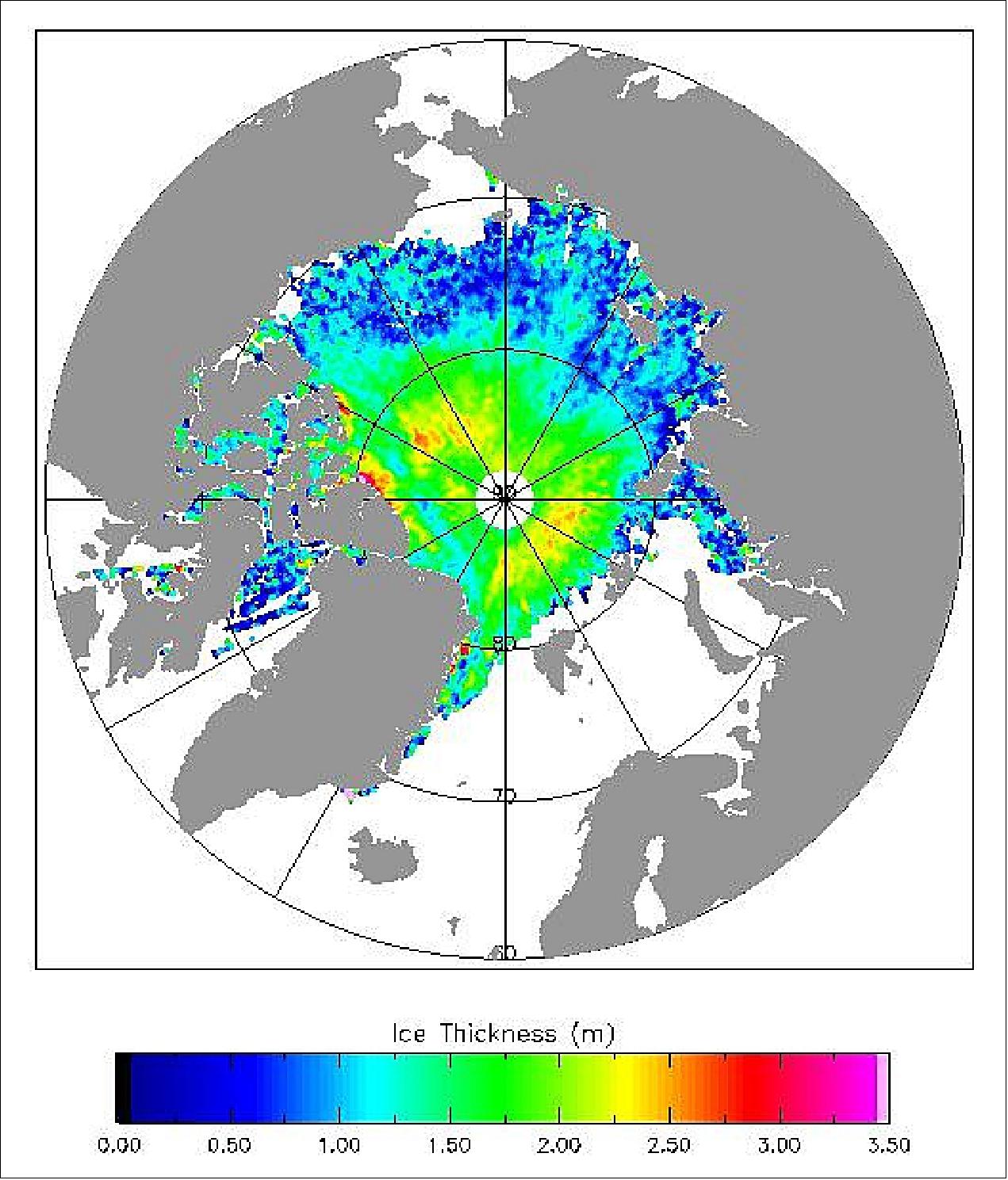
• July 20, 2015: Measurements from ESA’s CryoSat-2 satellite show that the volume of Arctic sea ice increased by a third following the unusually cool summer of 2013. This new finding suggests that ice in the northern hemisphere is more sensitive to changes in summer melting than it is to winter cooling. 74)
- Scientists at University College London (UCL) and the University of Leeds in the UK used 88 million sea-ice thickness measurements taken by CryoSat between 2010 and 2014. The study, published today in Nature Geoscience, shows a 14% reduction in the volume of summer sea ice between 2010 and 2012, but the volume of ice jumped by 41% in 2013, when the summer was 5% cooler than the previous year. Lead author Rachel Tilling, from CPOM (Centre for Polar Observation and Modelling) at UCL, said, “The summer of 2013 was much cooler than recent years, with temperatures typical of those seen in the late 1990s. “This allowed thick sea ice to persist northwest of Greenland because there were fewer days when it could melt. Although models have suggested that the volume of Arctic sea ice is in long-term decline, we know now that it can recover by a significant amount if the melting season is cut short.” 75)
- The team say although the first five years of CryoSat-2 measurements have revealed important information on the state of Arctic sea ice, the record is still short to establish a long-term trend. The team now plans to use the measurements of CryoSat-2 of changing sea-ice thickness to help improve the models that are used to predict future climate change, and also to assist maritime activities in the Arctic region, which can be dangerous and costly to navigate.
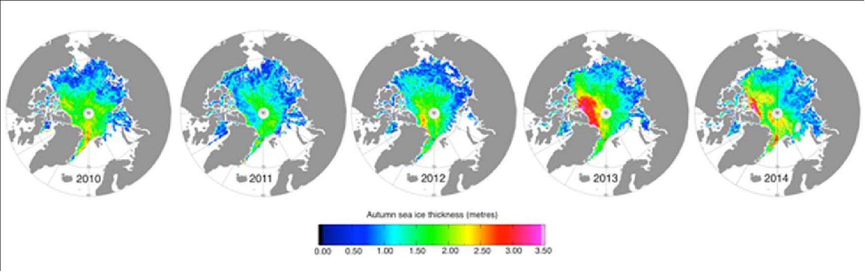
• May 22, 2015: A recent acceleration in ice loss in a previously stable region of Antarctica has been detected by ESA’s ice mission. The latest findings by a team of scientists from the UK’s University of Bristol show that with no sign of warning, multiple glaciers along the Southern Antarctic Peninsula suddenly started to shed ice into the ocean starting in 2009 at rate of about 60 km3 each year. 76)
- This makes the region one of the largest contributors to sea-level rise in Antarctica, having added about 300 km3 of water into the ocean in the past six years. Some glaciers along the coastal expanse are currently lowering by as much as four m each year. Prior to 2009, the 750 km-long Southern Antarctic Peninsula showed no signs of change.
- “It appears that sometime around 2009, the ice-shelf thinning and the subsurface melting of the glaciers passed a critical threshold that triggered the sudden ice loss,” said Bert Wouters from the University of Bristol, who led the study. “However, compared to other regions in Antarctica, the Southern Peninsula is rather understudied, exactly because it did not show any changes in the past, ironically.”
- The study includes five years of measurements from ESA’s ice mission, CryoSat-2, which employs an advanced radar altimeter that can measure the surface height variation of ice in fine detail, allowing scientists to record changes in its volume with unprecedented accuracy. The ice loss in the region is so large, that it has even caused small changes in Earth’s gravity field, detected by the US/German GRACE mission (Figure 68). — Climate models show that the sudden change cannot be explained by changes in snowfall or air temperature. Instead, the team attributes the rapid ice loss to warming oceans.
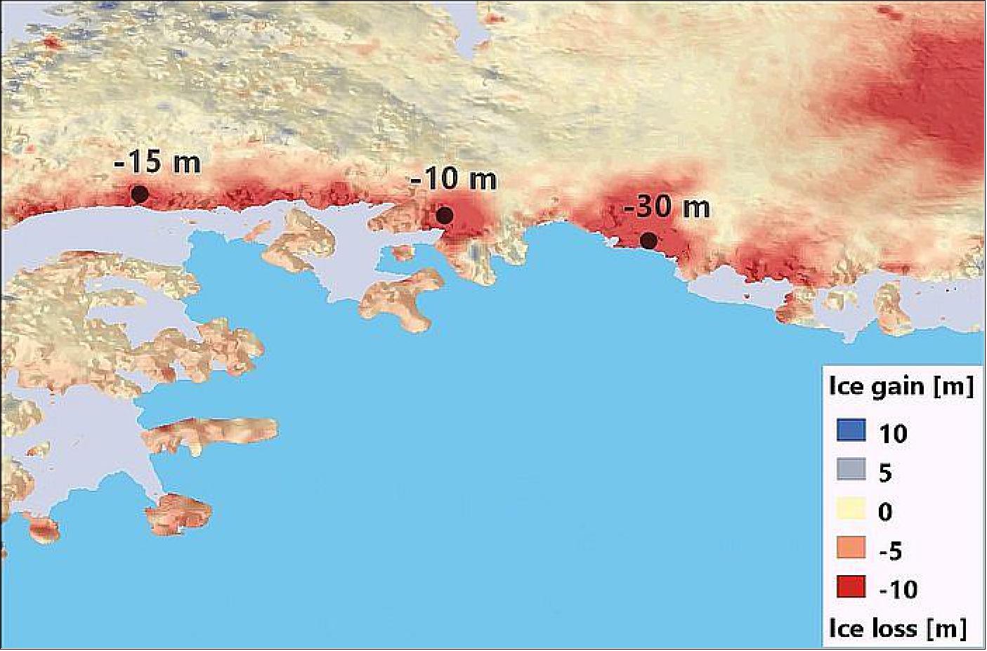
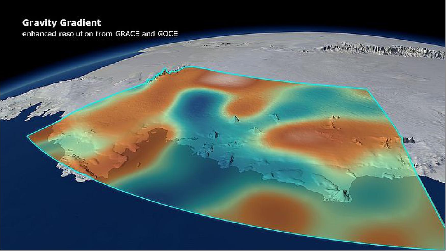
Legend to Figure 68: Changes in Earth’s gravity field resulting from loss of ice from West Antarctica between November 2009 and June 2012 (mE = 10–12 s–2). A combination of data from ESA’s GOCE mission and NASA’s GRACE satellites shows the ‘vertical gravity gradient change’.
• April 17, 2015: ESA’s ice mission has become the first satellite to provide information on Arctic sea-ice thickness in near-real time to aid maritime activities in the polar region. Marking five years in orbit On April 8, 2015, CryoSat-2 is the first mission to deliver complete maps of Arctic sea-ice thickness – a key indicator of global climate change and of the state of the Arctic itself. 77)
- With specialist data processing provided by the UK’s CPOM (Center for Polar Observation and Modelling), these measurements can now be delivered within two days of acquisition through a website launched today. 78)
- The rapid data processing is important for managing and planning activities affected by Arctic sea ice, such as shipping, tourism, Arctic exploration and search and rescue.
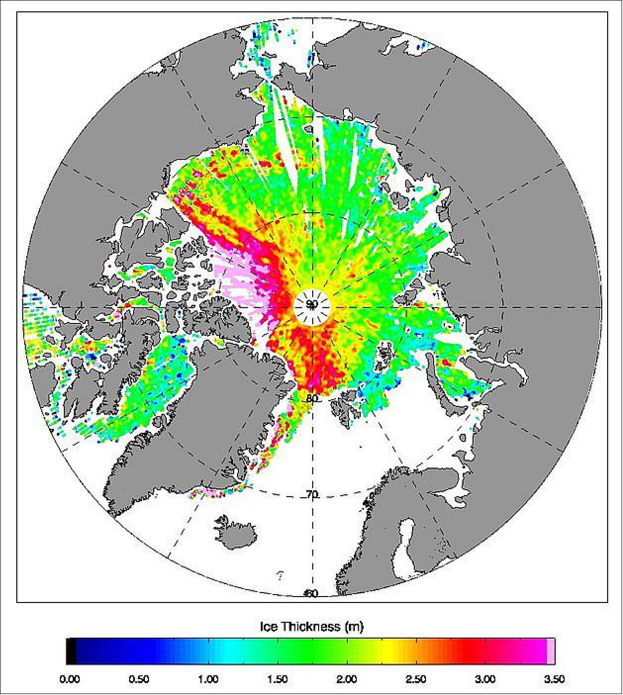
- “This new capability goes far beyond CryoSat’s original purpose, which was to collect measurements for scientific research,” said Professor Andy Shepherd, CPOM Director and the CryoSat’s principal scientific advisor. “The mission is now an essential tool for a wide range of services operating in areas of the planet where sea ice forms.”
- With the rapidly increasing economic growth in the Arctic, timely and routine information on sea-ice thickness will help to ensure that users of the Arctic can plan and carry out their operations safely and with care. The rapid access to data will also ease scientific research in the polar region, improving our understanding of how this sensitive environment is responding to climate change.
- The latest measurements available on the new website also show that sea ice around Norway’s Svalbard Archipelago is today only a meter thick – approximately half of what it was in the winter of 2011 just after CryoSat-2 was launched. The thinner ice around Svalbard coincides with a warming of the surrounding Barents Sea (Ref. 77).
• March 18, 2015: Trekking to the far reaches of the Arctic for the sole purpose of collecting snow and ice measurements may seem extreme, but it is thanks to these efforts that scientists will soon have even better satellite information at their fingertips to assess changes in polar ice. - Over the last year, the measurements made by scientists camping on the ice and from various aircraft during a month-long expedition have been painstakingly processed so that they can be used to confirm data from ESA’s CryoSat-2 ice mission. 79)
- CryoSat-2 measures the height of ice – both of that floating in the polar oceans and of the vast ice sheets covering Greenland and Antarctica. This information is essential for working out the thickness of the ice and how it is changing and, ultimately, how the volume of Earth’s ice is being affected by the climate. Given the crucial nature of understanding the links between ice and climate, it is important to make sure that CryoSat’s measurements remain accurate, even if this means heading out to one of the most inhospitable places on Earth.
- Scientists from numerous European and North American organizations volunteered to do just this. Their task was to take measurements of the Arctic sea ice using a suite of sensors on a different aircraft, as well as to measure snow and ice depth meticulously by hand on the ice – all the while keeping an eye out for polar bears. The ground team ranged from hardened polar scientists who wore jeans and took measurements with their bare hands despite temperatures of –30°C to PhD students, who had never experienced the harshness of an Arctic campaign.
- The campaign measurements actually go further than just validating the CryoSat-2 satellite data, they contribute significantly to the continuous improvement in the quality of ice-thickness maps. In fact, this latest Arctic expedition has played an important part in ESA’s upcoming CryoSat-2 data product release.
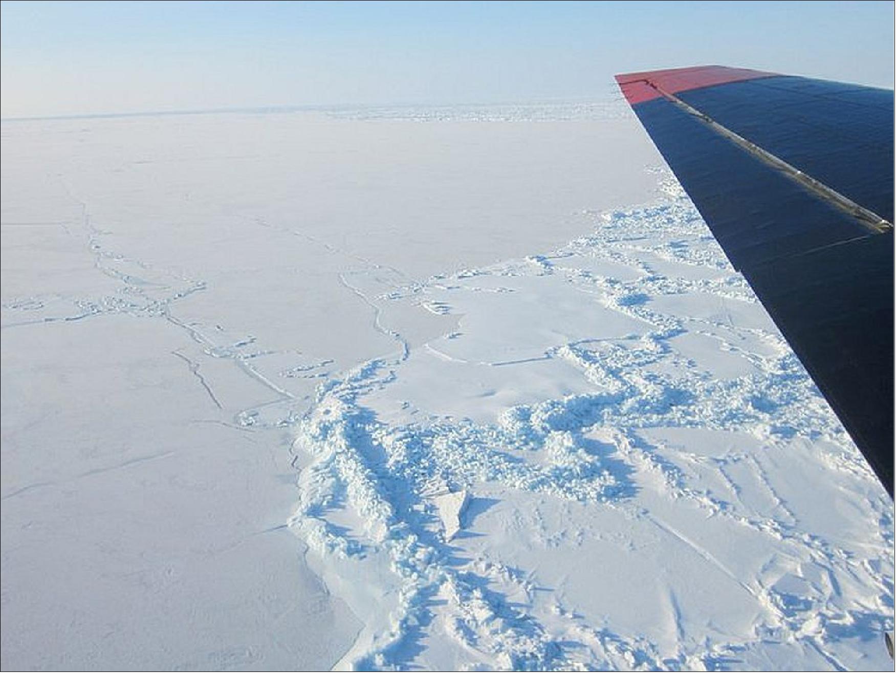
- From April, scientists will have, for the first time, access to systematic sea-ice ‘freeboard’ information with which to generate ice-thickness maps. Freeboard describes the height of sea ice protruding above the water line. Until now, scientists had to process the CryoSat-2 data to calculate this. Tommaso Parrinello, CryoSat-2 Mission Manager, said, “The validation aspect also indicates that the satellite is still in excellent health and providing precision data despite being in orbit for five years.” Malcolm Davidson, Head of ESA’s Earth Observation Campaigns, said, “We are using CryoSat to measure an extremely dynamic environment” (Ref. 79).
• January 23, 2015: Rapid ice loss in a remote Arctic ice cap has been detected by the Sentinel-1A and CryoSat satellites. Located on Norway’s Nordaustlandet island in the Svalbard archipelago, parts of the Austfonna ice cap have thinned by more than 50 m since 2012 – about a sixth of the ice’s thickness. 80)
- The research team, led by scientists from the Centre for Polar Observation and Modelling (CPOM) at the University of Leeds in the UK, used satellite observations to document rapid acceleration and ice loss from a formerly slow-flowing, marine-based sector of Austfonna, the largest ice cap in the Eurasian Arctic. During the past two decades, the sector ice discharge has increased 45-fold, the velocity regime has switched from predominantly slow (~ 101 m/yr) to fast (~ 103 m/yr) flow, and rates of ice thinning have exceeded 25 m/yr. At the time of widespread dynamic activation, parts of the terminus may have been near floatation. Subsequently, the imbalance has propagated 50 km inland to within 8 km of the ice cap summit. 81)
- Melting ice caps and glaciers are responsible for about a third of recent global sea-level rise. Although scientists predict that they will continue to lose ice in the future, determining the exact amount is difficult, owing to a lack of observations and the complex nature of their interaction with the surrounding climate. - There is evidence that the surrounding ocean temperature has increased in recent years, which may have been the original trigger for the ice cap thinning. Long-term observations by satellites are crucial for monitoring such climate-related phenomena in the years and decades to come.
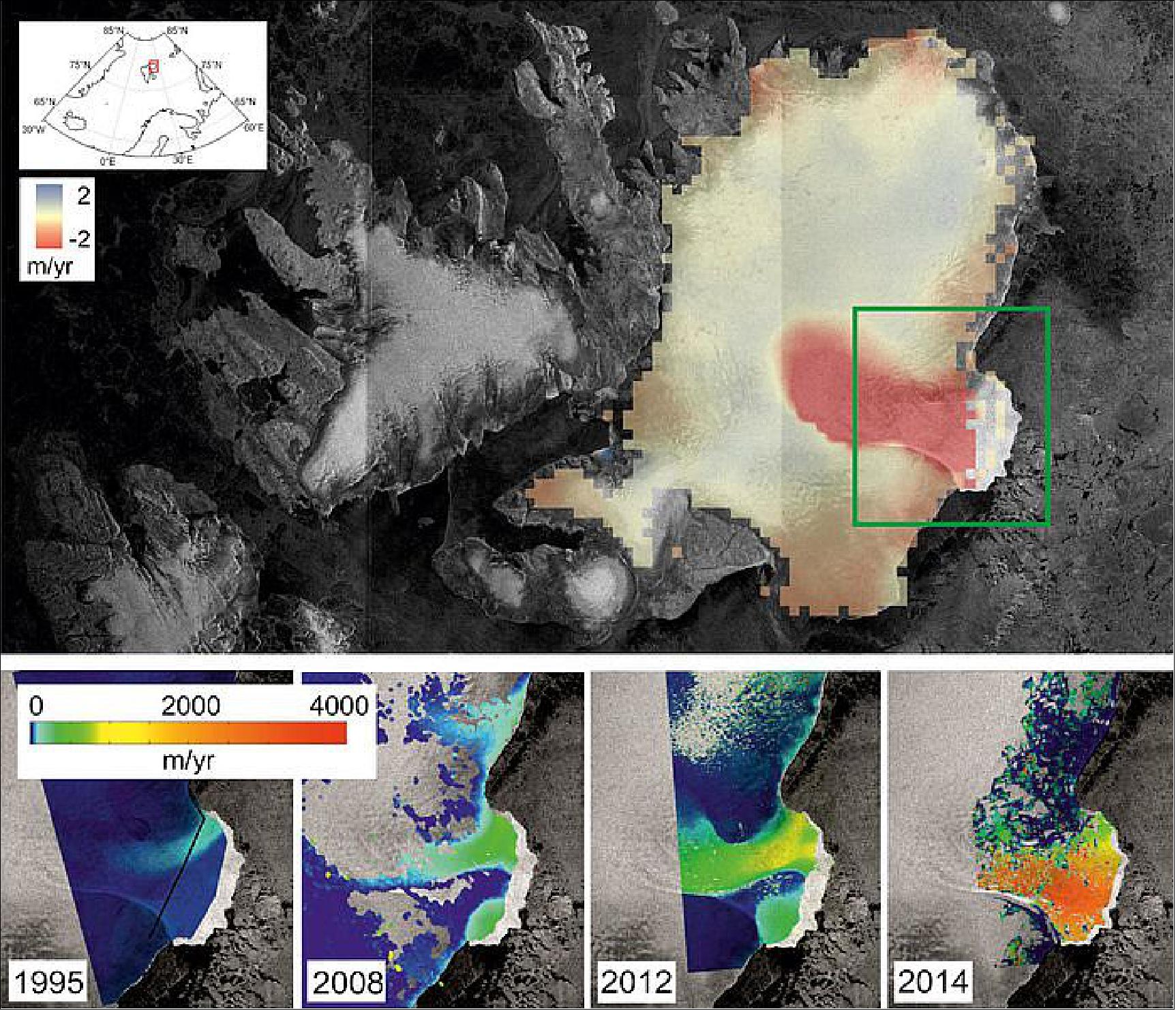
Legend to Figure 71: The main figure (top) shows the rate of ice cap elevation change between 2010 and 2014 observed by CryoSat, overlaid on an image acquired by Sentinel-1A (in 2014). Red indicates that the ice surface is lowering. In the southeast region (green box) ice thinning far exceeds the color scale of 2 m per year. - A closer look at the southeast region is shown in the four smaller figures below. These figures show the evolution of ice velocity over the last two decades. Ice velocity in 2014 was mapped using Sentinel-1A and the DLR (German Aerospace Center) TerraSAR-X mission.
• Dec. 15, 2014: CryoSat has delivered this year’s map of autumn sea-ice thickness in the Arctic, revealing a small decrease in ice volume. In a new phase for ESA’s ice mission, the measurements can now also be used to help vessels navigate through the north coastal waters of Alaska, for example: 82)
- Measurements made during October and November show that the volume of Arctic sea ice now stands at about 10,200 km3 – a small drop compared to last year’s 10,900 km3. The volume is the second-highest since measurements began in 2010, and the five-year average is relatively stable. This, however, does not necessarily indicate a turn in the long-term downward trend. — The analysis was made by a team of researchers at CPOM (Centre for Polar Observation and Modelling) at UCL (University College London), UK.
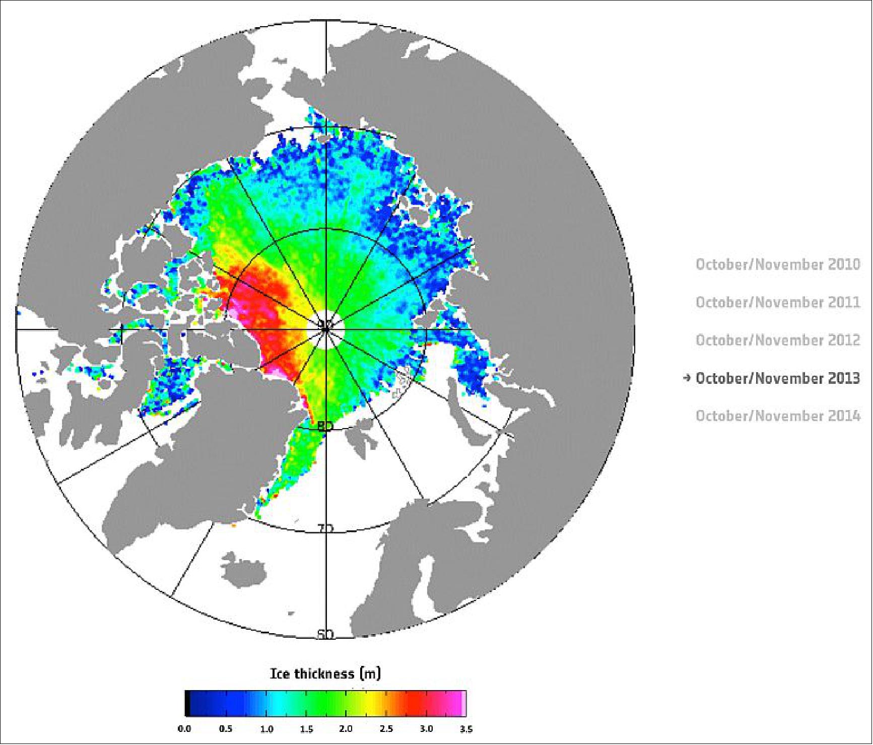
• Nov. 2014: The CryoSat-2 mission has recently been extended to the end of 2016. 83)
• October 3, 2014: Although the main task of ESA's CryoSat-2 mission is to measure the elevation of the world’s ice but its altimetry measurements acquired over oceans measure sea-surface height — the data of CryoSat-2 has also been used to create a new gravity map, exposing thousands of previously uncharted ‘seamounts’, ridges and deep ocean structures. This vivid new picture of the least-explored part of the ocean offers fresh clues about how continents form and breakup (Figures 73 and 74). 84)
Carrying a radar altimeter, CryoSat’s main role is to provide detailed measurements of the height of the world’s ice. This allows the project to see how the thickness of the ice changes, seasonally and in response to climate change. However, CryoSat-2 works continuously, whether there is ice below or not. This means that the satellite can also measure the height of the surface of the sea. These measurements can be used to create global marine gravity models and, from them, maps of the seafloor.
Although invisible to the eye, the sea surface has ridges and valleys that echo the topography of the ocean floor, but on a greatly reduced scale (i.e., the sea surface mimics the ocean floor). The effect of the slight increase in gravity caused by the mass of rock in an undersea mountain is to attract a mound of water several meters high over the seamount. Deep ocean trenches have the reverse effect (producing a dip on the sea surface). These features can only be detected by using radar altimetry from space. These features can only be detected by using radar altimetry from space.
Scientists from SIO (Scripps Institution of Oceanography) at UCSD (University California San Diego) used altimetry measurements from ESA’s CryoSat-2 mission and from the CNES–NASA Jason-1 satellite to create a new marine gravity map mirroring features of the ocean floor– twice as accurate as the previous version produced nearly 20 years ago. They used measurements of CryoSat-2 during the last 4 years as well as the measurements of Jason-1 during the last 12 years. The new maps offer geophysics new tools to investigate little-studied remote ocean basins and processes such as seafloor spreading. 85)
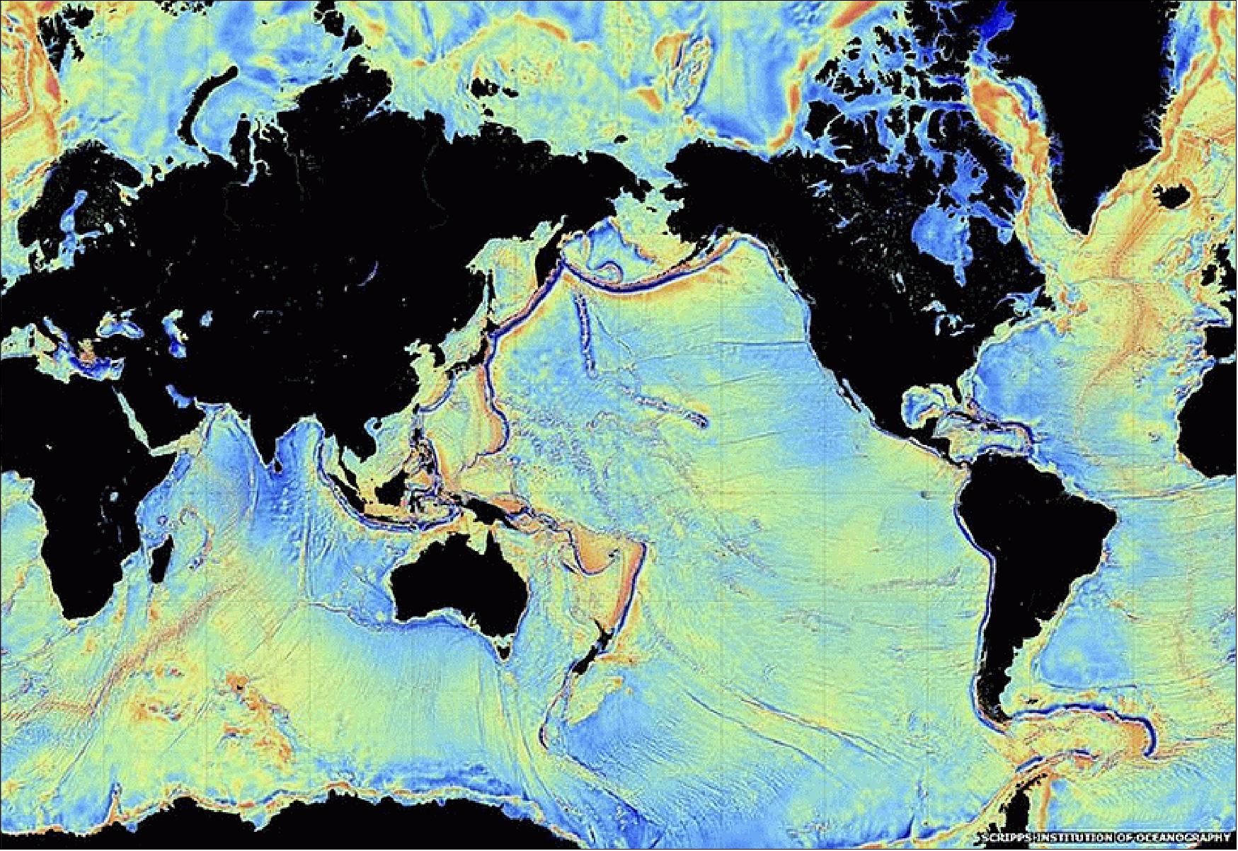
Previously unseen features in the map include newly exposed continental connections across South America and Africa, and new evidence for seafloor spreading ridges at the Gulf of Mexico that were active 150 million years ago and are now buried by layers of sediment more than a kilometer thick. One of the most important uses of this new marine gravity field will be to improve the estimates of seafloor depth in the 80% of the oceans that remains uncharted or is buried beneath thick sediment.
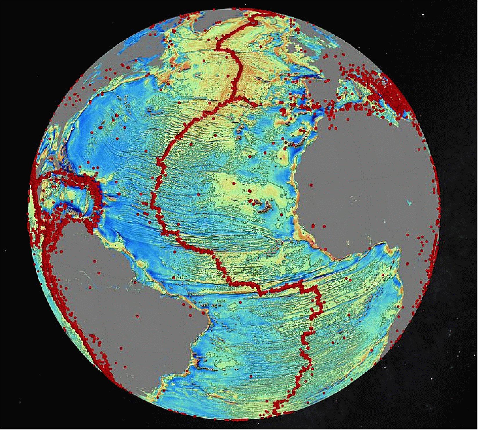
• August 20, 2014: Measurements from ESA’s CryoSat-2 mission have been used to map the height of the huge ice sheets that blanket Greenland and Antarctica and show how they are changing. New results reveal combined ice volume loss at an unprecedented rate of ~500 km3 a year. 86)
- The research was carried out by Germany’s Alfred Wegener Institute, Helmholtz Center for Polar and Marine Research. The results were published in The Cryosphere, a European Geosciences Union journal (Ref. 87).
This study focuses on the present-day surface elevation of the Greenland and Antarctic ice sheets. Based on 3 years of CryoSat-2 data acquisition, the team derived new DEMs (Digital Elevation Models) as well as elevation change maps and volume change estimates for both ice sheets. The accuracy of the derived DEMs for Greenland and Antarctica is similar to those of previous DEMs obtained by satellite-based laser and radar altimeters. Comparisons with ICESat data show that 80% of the CryoSat-2 DEMs have an uncertainty of less than 3 m ± 15 m. The surface elevation change rates between January 2011 and January 2014 are presented for both ice sheets. The team compared their results to elevation change rates obtained from ICESat data covering the time period from 2003 to 2009. The comparison reveals that in West Antarctica the volume loss has increased by a factor of 3. It also shows an anomalous thickening in Dronning Maud Land, East Antarctica which represents a known large-scale accumulation event. This anomaly partly compensates for the observed increased volume loss of the Antarctic Peninsula and West Antarctica. - For Greenland the team found a volume loss increased by a factor of 2.5 compared to the ICESat period with large negative elevation changes concentrated at the west and southeast coasts. The combined volume change of Greenland and Antarctica for the observation period is estimated to be -503 ± 107 km3 yr-1. Greenland contributes nearly 75% to the total volume change with -375 ± 24 km3 yr-1. 87)
The new maps, which incorporate 7.5 million elevation measurements of Greenland and 61 million of Antarctica collected by CryoSat-2 in 2012, are the most complete to date from a single satellite mission.
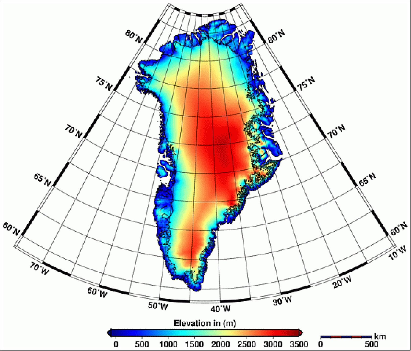
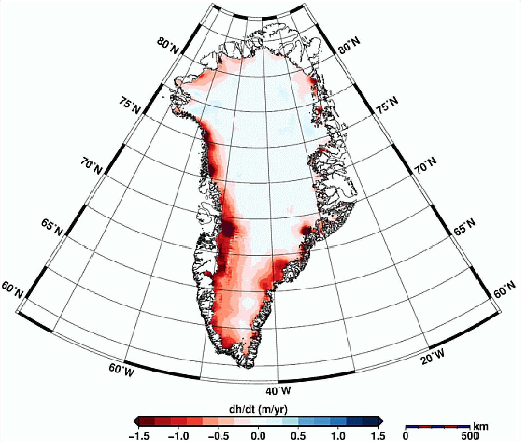
Legend to Figure 76: Using 14.3 million measurements collected by ESA’s CryoSat-2 mission between January 2011 and January 2014, the research team from the Alfred Wegener Institute has discovered that the Greenland ice sheet is shrinking in volume by 375 km3 a year.
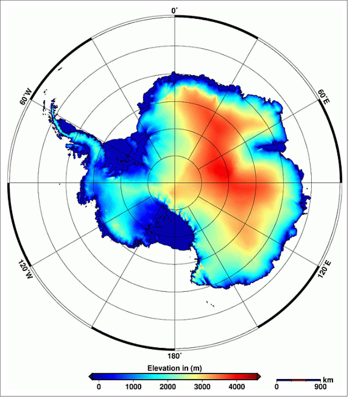
Legend to Figure 77: This new elevation model of Antarctica incorporates 61 million measurements from ESA’s CryoSat-2 satellite collected throughout 2012. The edge of the ice sheet is outlined in black.
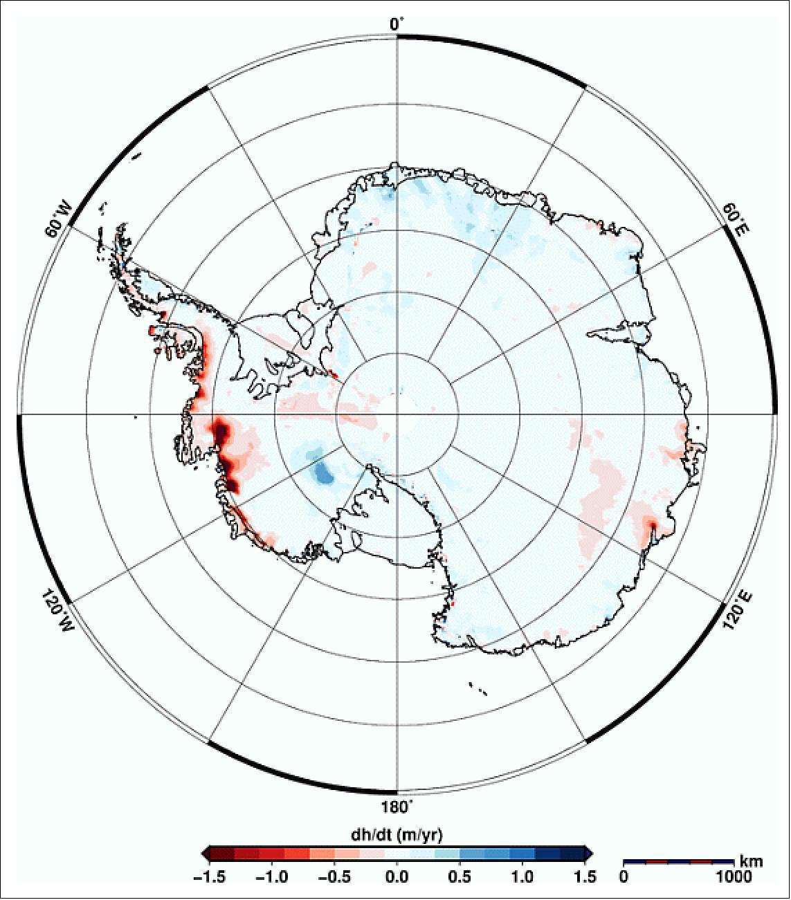
Legend to Figure 78: Using 200 million measurements collected by ESA’s CryoSat-2 mission between January 2011 and January 2014, the research team from the Alfred Wegener Institute has discovered that the Antarctic ice sheet is shrinking in volume by 125 km3 a year.
• May 19, 2014: Three years of observations from ESA’s CryoSat-2 satellite show that the Antarctic ice sheet is now losing 159 billion tons of ice each year – twice as much as when it was last surveyed. The polar ice sheets are a major contributor to the rise in global sea levels, and these newly measured losses from Antarctica alone are enough to raise global sea levels by 0.45 mm each year. 88) 89)
- These latest findings by a team of scientists from the UK’s CPOM (Centre for Polar Observation and Modelling) show that the pattern of imbalance continues to be dominated by glaciers thinning in the Amundsen Sea sector of West Antarctica. Between 2010 and 2013, West Antarctica, East Antarctica and the Antarctic Peninsula lost 134, 3, and 23 billion tons of ice each year, respectively (note: 1 billion tons of ice, or 1 Gt, is equivalent to ~1 km3 of ice). The average rate of ice thinning in West Antarctica has increased compared to previous measurements, and this area’s yearly loss is now one third more than measured over the five years before the launch of CryoSat-2.
- CryoSat surveys almost all – 96% – of the Antarctic continent, reaching to within 215 km of the South Pole. In addition, it has increased coverage over coastal regions, where today’s ice losses are concentrated.
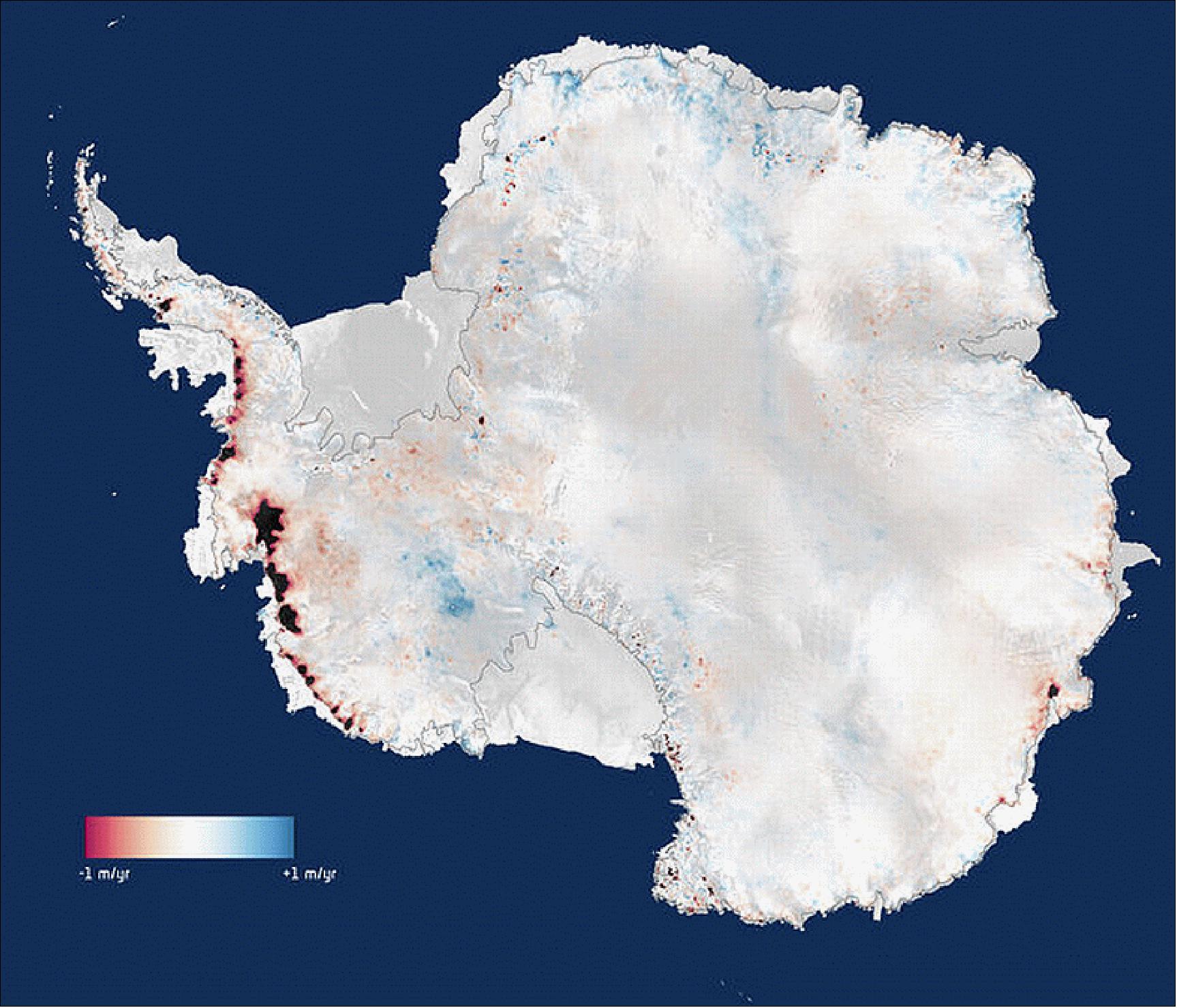
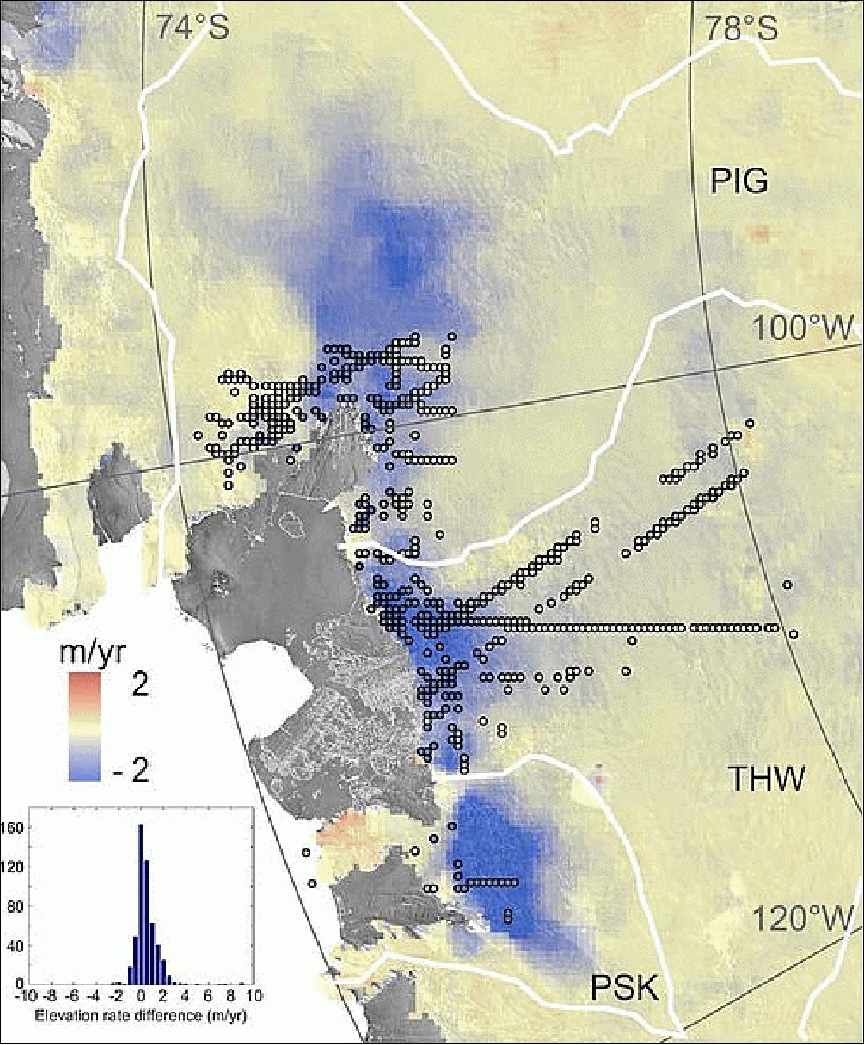
- A US article by NASA/JPL and UCI (University of California, Irvine), being published in Geophysical Research Letters of AGU, comes to the same conclusions as their British colleagues. 90) The findings of the study were also presented at a NASA press conference on May 12, 2014. 91)
The study finds a rapidly melting section of the West Antarctic Ice Sheet appears to be in an irreversible state of decline, with nothing to stop the glaciers in this area from melting into the sea. The study presents multiple lines of evidence, incorporating 40 years of observations that indicate the glaciers in the Amundsen Sea sector of West Antarctica "have passed the point of no return," according to glaciologist and lead author Eric Rignot, of UC Irvine and NASA's Jet Propulsion Laboratory (JPL) in Pasadena, California. These glaciers already contribute significantly to sea level rise, releasing almost as much ice into the ocean annually as the entire Greenland Ice Sheet. They contain enough ice to raise global sea level by 1.2 m and are melting faster than most scientists had expected. Rignot said these findings will require an upward revision to current predictions of sea level rise.
The team used radar observations captured between 1992 and 2011 by the European Earth Remote Sensing (ERS-1 and -2) satellites to map the grounding lines' retreat inland. The satellites use a technique called radar interferometry, which enables scientists to measure very precisely — within less than a quarter of an inch — how much Earth's surface is moving. Glaciers move horizontally as they flow downstream, but their floating portions also rise and fall vertically with changes in the tides. Rignot and his team mapped how far inland these vertical motions extend to locate the grounding lines. The accelerating flow speeds and retreating grounding lines reinforce each other. As glaciers flow faster, they stretch out and thin, which reduces their weight and lifts them farther off the bedrock. As the grounding line retreats and more of the glacier becomes waterborne, there's less resistance underneath, so the flow accelerates.
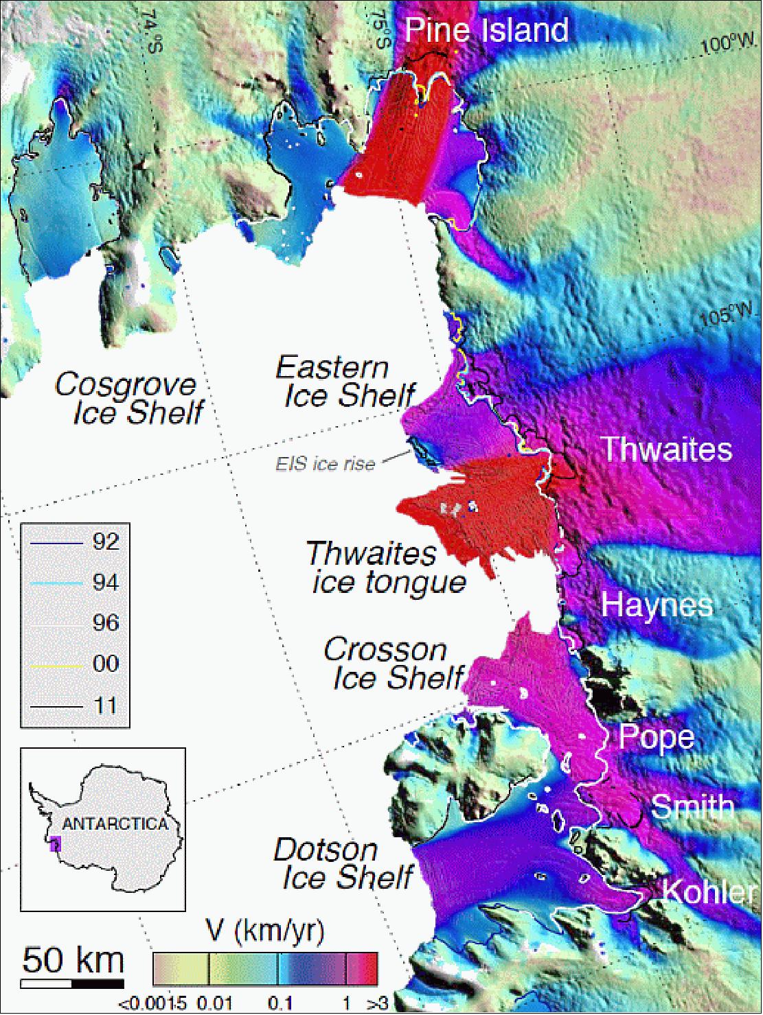
Legend to Figure 81: Interferometrically-derived grounding lines of the glaciers are shown in color code for years 1992, 1994, 1996, 2000 and 2011, with glacier and ice shelf names. Note that for Pine Island and Smith/Kohler, the Figure merges two independent differential interferograms to show a more complete spatial coverage of grounding lines.
• In April 2014, Cryosat-2 achieved four years of operations, covering six-months of commissioning and the follow on routine operations. Overall, the mission has proven to be very successful and the spacecraft overall performance very reliable. As CryoSat-2 completes its fourth year on orbit, unit ageing is being closely monitored by the FCT (Flight Control Team). CryoSat-2 has achieved over 20,000 orbits in flight and with the current power and fuel margins it is highly likely that the satellite would be able to continue well beyond the currently planned end of mission date, in 2016. 92)
- Debris collision monitoring: Space debris has become, and continues to be, a collision risk for orbiting satellites. At the CryoSat-2 operational orbit height of 717km this risk is such that the FCT has put in place a CAM (Collision Avoidance Maneuver) protocol. On reception of close approach conjunction warnings, the CryoSat-2 satellite can be maneuvered out of the way of the piece of debris.
The warnings generated by both the ESA Space Debris Office (SDO) CRASS system and with support from the US JSpOC (Joint Space Operations Center) provide details of the predicted conjunctions between CryoSat-2 and all other tracked LEO objects. These warnings specify the conjunction times, geometries, miss distances, orbit prediction errors and probabilities of the events. This data needs to be analyzed by the FCT, FD (Flight Dynamics) and SDO and a decision on whether to maneuver or not needs to be taken – sometimes at very short notice i.e. within 24 hours.
The conjunction encounters experienced by CS-2 to date have been varied and not always deterministic with debris items including Iridium clouds, COSMOS and the Fengyun-1C debris. Dedicated CAMs have been carried out in a couple of cases interrupting routine operations and collection of Science data. In other cases it has been possible to combine the collision avoidance maneuver with a planned OCM (Orbit Control Maneuver), by slightly changing the timing or parameters of the OCM.
Date | Chaser | Miss distance | PCOL | Warning notice | Actions |
Oct. 2, 2010 | Thor Ablestar fragmentation debris | 24 m radial | 2.3 x 10⁻³ | ~41 hours | Head-on approach geometry. CAM executed. Initial antiflight direction maneuver followed by in flight maneuver to return to nominal ground track |
May 17, 2012 | Cosmos-2251 debris | -73m radial | 3.18 x 10⁻⁶ | 6 days | Head-on approach geometry. Inflight direction maneuver. Nominal planned OCM executed which mitigated the conjunction. |
Aug. 13, 2012 | Cosmos-2251 debris | -81 m radial | 1.2 x 10⁻¹⁶ | < 24 hours | Lateral approach geometry. Inflight direction maneuver. Combined collision avoidance/orbit maintenance maneuver. |
Oct. 11, 2013 | Fengyun-1C debris | -6 m radial | 3.65 x 10⁻⁴ | < 48 hours | Head-on approach geometry. Ground track orbit maintenance maneuver executed as planned increasing radial miss distance and reducing the probability of the chaser. Combined collision avoidance/orbit maintenance maneuver. |
Oct. 15, 2013 | Fengyun-1C debris | 5 m radial | 3.67 x 10⁻³ | < 3 days over weekend | Head-on approach geometry. CAM executed. Initial inflight direction maneuver followed by antiflight maneuver to return to nominal ground track. |
Jan. 9, 2014 | India PSLV debris | -114 m radial | 1.74 x 10⁻⁸ | 4 days over weekend | Lateral approach geometry. Inflight direction maneuver. Large uncertainties in drag conditions. Routine OCM executed half an orbit before conjunction event to increase radial miss distance. |
- Roll maneuver campaigns over ocean for calibration: A roll maneuver campaign was devised to support the need to characterize the interferometer performance and in addition to determine the extent of thermally induced bending on the SIRAL Antenna bench. The CS-2 roll maneuver campaigns have been supported during commissioning and additionally in Oct. 2011, Sept. 2012, Sept .2013 and with the last campaign in Jan. 2014. The specification for the rolled SARIn measurements is that they take place over ocean for calibration of science data, away from the South Atlantic Anomaly (spacecraft constraint to ensure stable STR behavior), and to be repeated yearly (every 369 days) and for the last campaign one solar cycle apart (480 days) using the same orbit segments. The data takes need to occur during both eclipse and sunlight periods (if possible), covering ascending and descending passes and over different oceans (Pacific and Indian) to ensure a complete set of the varied thermal conditions (Ref. 92).
- Support to IceBridge, CryoVEx Campaigns: As part of the nominal CryoSat-2 support to users the FCT aims to maintain maximum SIRAL availability and minimal loss of science data. In the case of support to NASA’s operation IceBridge and ESA’s CryoVEx (Cryosat Validation Experiment) type campaigns which occur every one or two years, the FCT aims to avoid possible SIRAL outages over the known underflight periods. These underflights are simply flown to match the time and groundtrack of the CryoSat-2 orbit (Ref. 92).
- Space segment improvements - MMFU Storage Capacity increase: CryoSat-2 operates fairly close to the limits with regard to the on board storage capacity of science data. The current scenario is that with the loss of one badly timed ground station pass, the packet stores can be over written. The CryoSat-2 MMFU (Mass Memory and Formatting Unit ) was originally designed with a spare 32 Gbit, one complete Partition. Analysis was conducted considering the spacecraft and ground segment activities required to increase the MMFU storage capacity to make use of the currently spare 32 Gbit. Simulations were carried out where the extra 32 Gbit were allocated between Packet Store (PS) 1 and PS2 (used to store the SAR and SARIn data) to try to minimize data loss in case of missed ground-station passes before or after a long blind orbit period. The simulations showed that the new PS sizes would allow to cope with a missed pass before or after the blind orbits period without a data loss. For the cases of more than one missed pass even the use of the complete memory cannot prevent data loss but does minimize it. The spacecraft activities needed to implement this change require the powering up of the remaining MMFU partition and to configure the PS1 and PS2 to the new recommended sizes. The SIRAL instrument would need to be Standby throughout this period with an expected outage of at least 2 orbits. Planning for execution of this activity is underway with the dates to be selected outside of the northern hemisphere winter to avoid gaps in science data at the most important ice monitoring times of the year.
- STR Enhanced software for Attitude Update mode: A proposal to update the STR (Star Tracker) Attitude Update mode to account for noisier CCDs at higher temperatures is being considered. As the STR CCDs age, they become more susceptible to thermal effects. CryoSat-2 needs to operate at certain times of the year with warm STRs . To ensure the longevity of the CryoSat-2 operations, the ageing STRs need to continue to work at these warm temperatures. The patches recently received cover enhancements of the IA (Initial Acquisition) mode of the STRs. The idea for further improvements cover possible updates to the AU (Attitude Update) mode of the STRs. One proposal is for the centroiding algorithm to be further enhanced to filter out false stars. Single bright pixels are already filtered out but further improvements could be made. A number of proposals have been put forward and the solution most suited to CryoSat-2 STRs needs to be further assessed.
- Long term performance monitoring: The CryoSat-2 subsystem battery management has been established around the eclipse seasons to optimize the battery capacity as the battery ages. The procedure now in operation was agreed and assessed together with Industry allowing simple rules to be put in place to modify the battery EOC (End of Charge) levels going into and coming out of the longest eclipse periods. The solution chosen was a simple seasonal commanding from ground, based on the observed behavior of the battery voltages. With the minimum battery voltage decreasing (i.e. going into a deeper period of eclipses), as soon as the battery voltage hits a predefined level, the EOC level is increased by one setting. The reverse logic is used as CryoSat-2 emerges from the deeper period of eclipses i.e. with the minimum battery voltage increasing, when the battery minimum voltage is greater than a predefined level for three consecutive days, the EOC levels can be decreased back to the original value. As the mission goes on, these EOC levels will be adjusted to suit the performance seen from the batteries. The management of the EOC levels ensures that the battery is always sufficiently charged to withstand a worst case safe mode entry and recovery, but is also not over charged, which would shorten the lifetime of the unit.
- New payload data applications: The primary mission goals of CryoSat-2 are to determine regional and basin-scale trends in perennial Arctic sea ice thickness and mass, and to determine regional and total contribution to global sea-level of the Antarctic and Greenland ice sheets. — CryoSat-2 is now providing high quality data to several user scientific communities: sea-ice, land-ice, meteorology, ocean, marine gravity, coastal zone and hydrology (Ref. 92).
• March 26, 2014: Water from melting glaciers and ice sheets, along with thermal expansion of ocean water due to rising temperatures, are causing global sea-level rise. Scientists are exploiting satellite data to understand better just how much each component contributes to this devastating consequence of climate change. The latest estimates show that global sea level is rising by about 3 mm a year, and this is one of the major threats of global warming, especially for low-lying coastal areas. 93)
Identifying the individual contributors to sea-level rise is one of the most complicated challenges in climate science. This involves tracking water as it moves in all its forms – solid, liquid or gas – around Earth. While Earth-observing satellites continuously map global and regional sea-level change, they can also be used to quantify the amount of water coming from various sources.
Under ESA’s Climate Change Initiative (CCI), experts in the domains of oceans, land, atmosphere and the cryosphere are working together to quantify the various sources of sea-level change – known as balancing the sea-level budget.
Changes in the mass of ice sheets and glaciers can be mapped using satellite radar altimeters, like the one flying on ESA’s CryoSat-2 that was specially designed to survey ice. By monitoring these changes, scientists can gage how much water they contribute to the ocean.
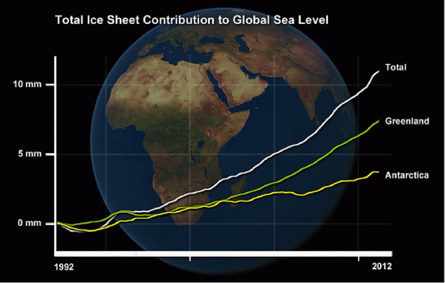
Legend to Figure 82: The rate of ice loss in Greenland and Antarctica is increasing. From 1992 to 2012, the two ice sheets contributed a total of 11.1 mm to global sea levels. This is about 20% of all sea-level rise over that 10-year period (Ref. 93).
• Feb. 2014: CryoSat-2 completed its first three years of operations on Nov. 19, 2013 when the spacecraft was declared operational. It continues to work flawlessly, acquiring and generating science data systematically, to measure the variation of sea-ice mass floating in the Arctic and trend of land-ice volume over Greenland and Antarctica. An issue affecting the onboard power system forced operations to fall back to the redundant system with little impact on the science retrieval. 94)
• Feb. 2014: Regarding collision avoidance, CryoSat-2 experienced seven conjunctions within 300 m in 2013, two required evasive maneuvers: 95)
- Oct. 11, 2013 (JSpOC alert): conjunction at ~340 m (53 m radial)
- Oct. 15, 2015 (JSpOC alert): conjunction at ~205 m (200 m radial).
• The CryoSat-2 spacecraft and its payload are operating nominally in 2014.
• January 2014: Near the center of Antarctica, measurements from CryoSat-2 show an unusual pattern in the ice sheet’s elevation (Figure 83). Scientists have now found the reason for this pattern – and the discovery is leading to even more accurate measurements from ESA’s ice mission. 96)
CryoSat collects data over Antarctica while passing on northbound and southbound orbits. But the data show an unusual pattern of height differences where these orbit cross, radiating from the South Pole.
Initially it was reasoned that there could be an issue with the satellite itself, such as a miscalculation of the altitude, a timing error or a problem with one of the corrections we apply to the measurements. - After eliminating the possibility of these errors through careful experimentation, scientists discovered that the pattern was caused by the way the satellite signal is scattered from the ice sheet surface.
Antarctica has some of the strongest and most persistent winds on Earth, which leave permanent erosional and depositional features on the surface and in the snow pack. The scientists found that these wind-driven features modify CryoSat-2’s radar measurements in such a way as to produce the pattern that has been detected. - The pattern in Figure 83 is not an ‘error’, but an artefact arising from the interaction of the polarization of CryoSat’s antenna with the structure of the ice surface induced by wind.
It has long been known that wind-driven directional properties of the ice sheet surface can affect the signal received by radar altimeters, but has never been seen so clearly. The most striking feature of the pattern – the diamond ring pattern close to the pole – had not been seen by past altimeter missions because they did not fly far enough south.
Since the pattern appears to be stable over time, the data can easily be corrected, ensuring that CryoSat’s past and future measurements of Antarctica are precise. The discovery also helps scientists better understand the interaction between radar waves and ice sheet surfaces.
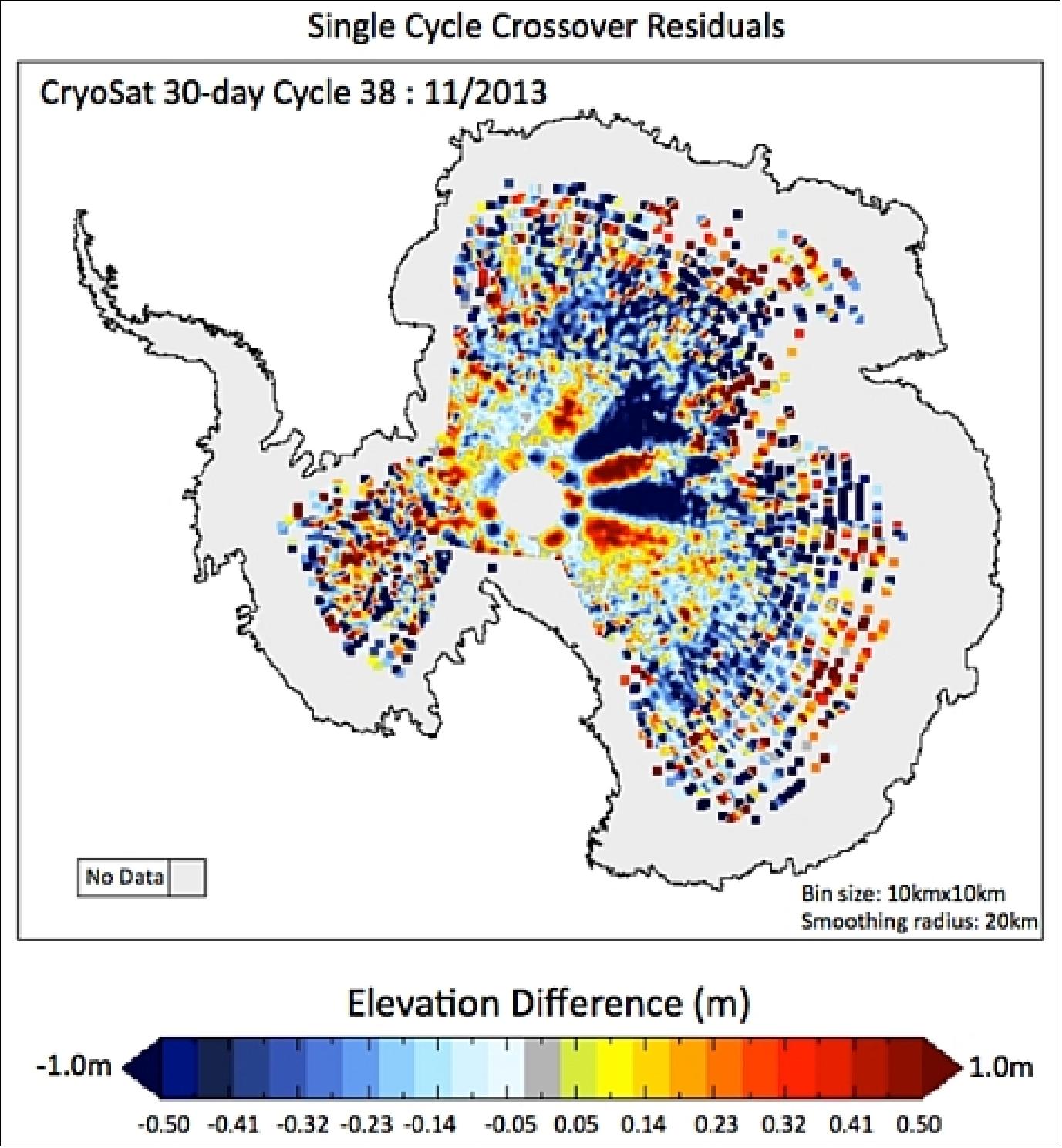
Legend to Figure 83: There is a distinct pattern of alternating high and low elevations (shown in red and blue), which inverts closer to the South Pole. After careful analysis, it was discovered that this is an artefact caused by the interaction of the polarization of CryoSat’s antenna with the structure of the ice.
• December 16, 2013: Measurements from CryoSat-2 show that the volume of Arctic sea ice has significantly increased this autumn. In October 2013, CryoSat-2 measured about 9000 km3 of sea ice – a notable increase compared to 6000 km3 in October 2012. This year’s multi-year ice is now on average about 20%, or around 30 cm, thicker than last year. While this increase in ice volume is welcome news, it does not indicate a reversal in the long-term trend. - It’s estimated that there was around 20 000 km3 of Arctic sea ice each October in the early 1980s, and so today’s minimum still ranks among the lowest of the past 30 years. 97)
• December 11, 2013: Three years of observations by ESA’s CryoSat-2 satellite show that the West Antarctic Ice Sheet is losing over 150 km3 of ice each year – considerably more than when last surveyed. The imbalance in West Antarctica continues to be dominated by ice losses from glaciers flowing into the Amundsen Sea. The ice thinning continues to be most pronounced along fast-flowing ice streams of this sector and their tributaries, with thinning rates of between 4–8 m per year near to the grounding lines – where the ice streams lift up off the land and begin to float out over the ocean – of the Pine Island, Thwaites and Smith Glaciers. 98)
The melting of ice sheets that blanket Antarctica and Greenland is a major contributor to global sea-level rise. An international team of polar scientists had recently concluded that West Antarctica caused global sea levels to rise by 0.28 mm each year between 2005 and 2010, based on observations from 10 different satellite missions. But the latest research from CryoSat-2 suggests, that the sea level contribution from this area is now 15% higher.
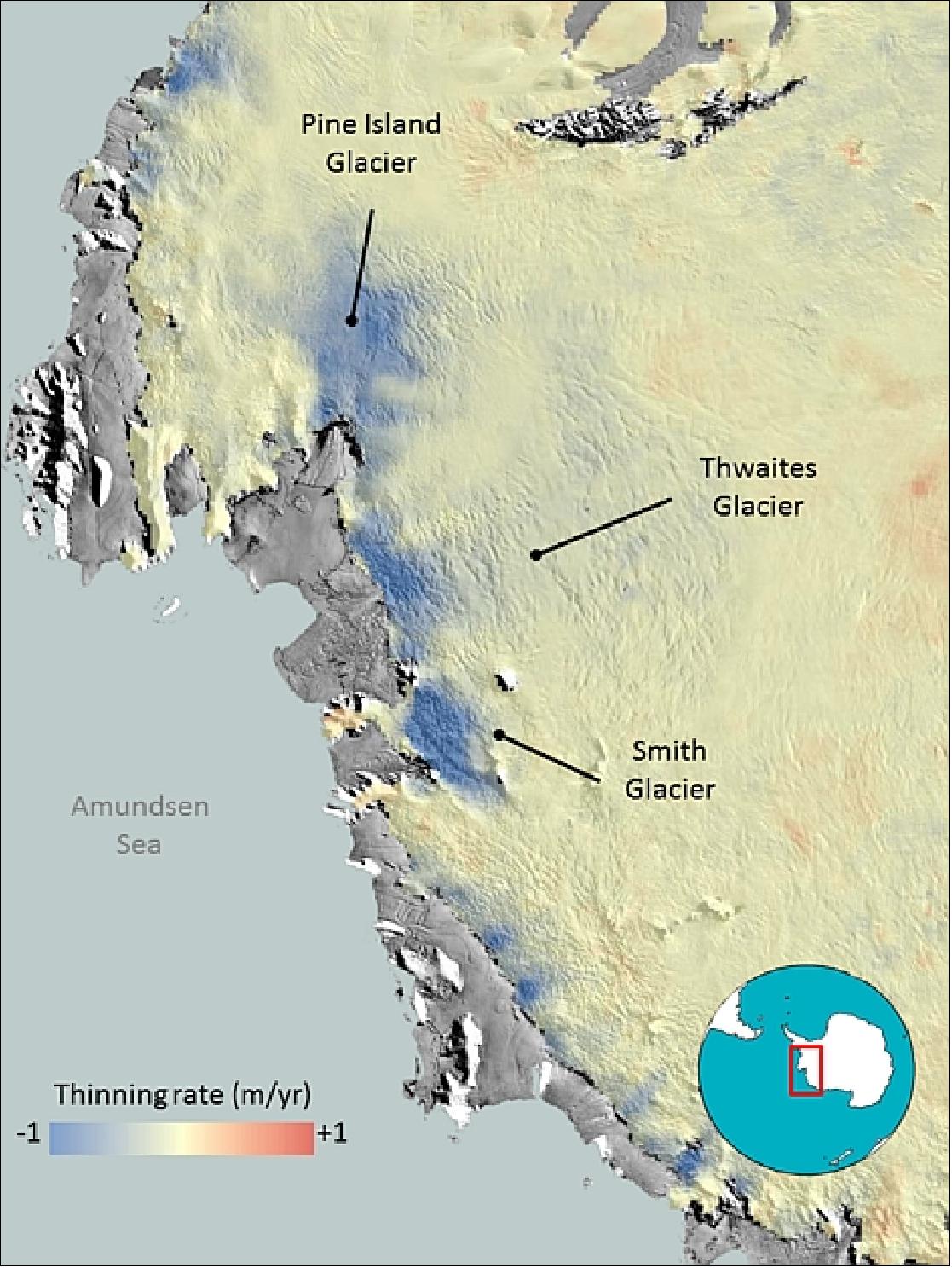
• During December 5-6, 2013, a major storm passed through northern Europe causing flooding, blackouts, grounding flights and bringing road, rail and sea travel to a halt. ESA’s CryoSat-2 satellite measured the storm surge from the recent North Sea storms, as high waters passed through the Kattegat sea between Denmark and Sweden. Since the storm coincided with a period of high tides in the North Sea, there were extremely high sea levels – a ‘storm surge’. In the UK, sea levels were at their highest since the 1953 North Sea Floods, while in Germany, parts of Hamburg were flooded. 99)
- On Dec. 6, CryoSat-2 passed over the Kattegat, providing an estimate of total water levels. The observations matched predictions, helping to confirm these models. The measurements were made by CryoSat’s radar altimeter that – although designed to measure sea-ice thickness – is providing outstanding results over sea and, especially, coastal areas.
- Until recently, altimeter measurements of sea-level height could only be made over open oceans, because of land interference closer to the coast. In the last few years, however, progress has been made in reducing these effects, also thanks to the new generation of radar altimeters being heralded by CryoSat-2. This has allowed scientists not only to map water levels closer to the coast, but also profile land surfaces and inland water targets such as small lakes, rivers and their intricate tributaries.
- Altimeter measurements from space can be used to validate storm surge models as well as provide near-realtime information that can be incorporated into predictions. Under ESA’s Data User Element, the 'eSurge' project is helping to optimize the use of altimetry and other types of satellite data to improve storm surge forecasting.
• Sept. 2013: CryoSat-2 has been in orbit since 2010 and with the satellite still in excellent health it is now set to continue providing precision measurements until 2017.
ESA’s CryoSat-2 mission has provided three consecutive years of Arctic sea-ice thickness measurements, which show that the ice continues to thin. Along with observations of ice extent, The measurements of CryoSat-2 thickness now span from October 2010 to April 2013, allowing scientists to work out the real loss of ice, monitor seasonal change and identify trends. CryoSat-2 continues to provide clear evidence of diminishing Arctic sea ice. 100)
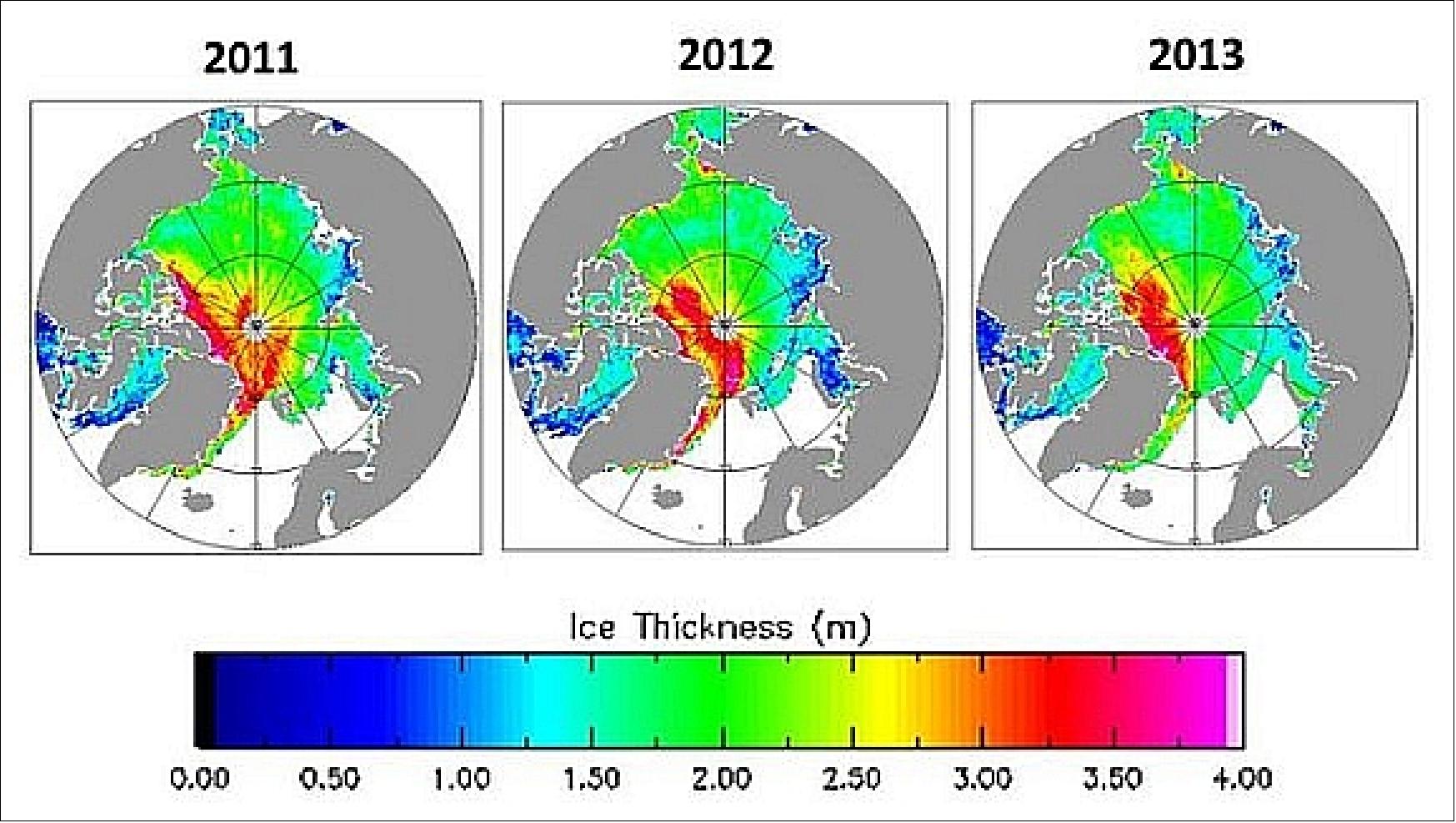
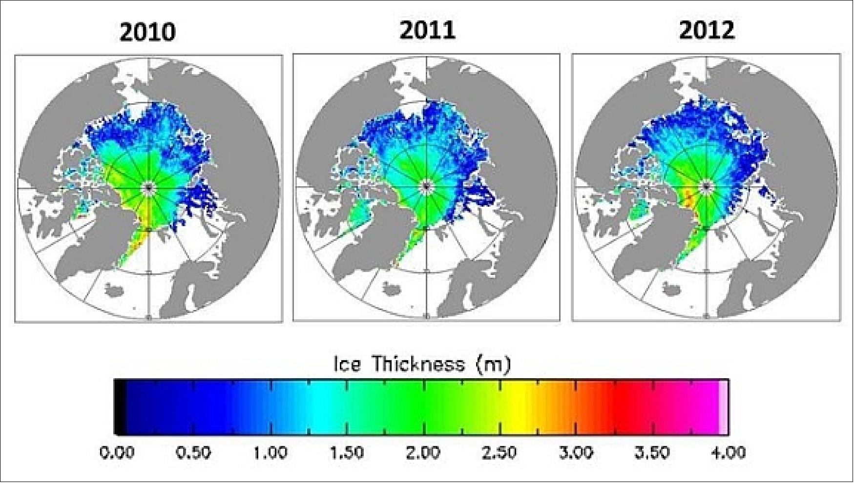
• In early July 2013, ESA is reporting that CryoSat-2 has found a vast crater in Antarctica’s icy surface. Scientists believe the crater was left behind when a lake lying under about 3 km of ice suddenly drained. 101)
Far below the thick ice sheet that covers Antarctica, there are lakes of fresh water without a direct connection to the ocean. These lakes are of great interest to scientists who are trying to understand water transport and ice dynamics beneath the frozen Antarctic surface – but this information is not easy to obtain.
By combining new measurements acquired by CryoSat-2 with older data from NASA’s ICESat satellite, the Cryosat team has mapped the large crater left behind by a lake, and even determined the scale of the flood that formed it.
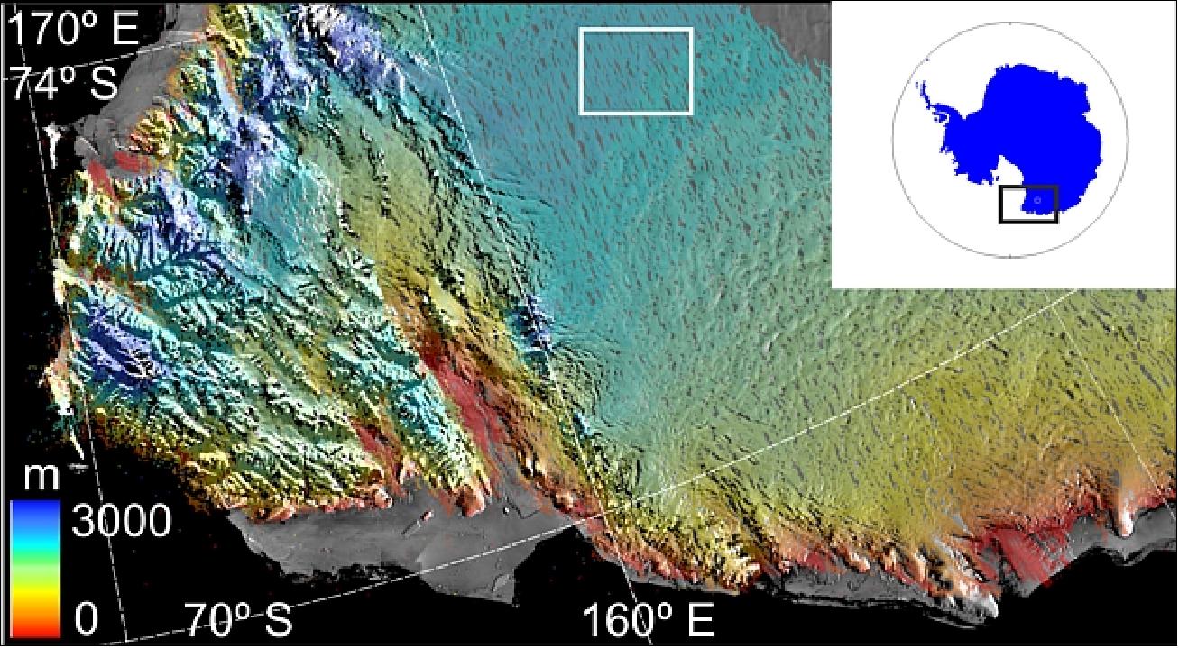
The CryoSat science team analyzed the data acquired by the SIRAL (SAR Interferometer Radar Altimeter) instrument on CryoSat-2 and demonstrated its novel capability to track topographic features on the Antarctic Ice Sheet. The perimeter and depth of a 260 km2 surface depression was mapped above an Antarctic SGL (Subglacial Lake) and, in combination with ICESat laser altimetry data,the decadal changes were charted in SGL volume. During 2007-2008, between 4.9 and 6.4 km3 of water drained from the SGL, and the peak discharge exceeded 160 m3/s. The flood was twice as large as any previously recorded, and equivalent to ~ 10 % of the meltwater generated annually beneath the ice sheet. - The ice surface has since uplifted at a rate of 5.6 ± 2.8 m/yr. Our study demonstrates the ability of CryoSat-2 to provide detailed maps of ice sheet topography, its potential to accurately measure SGL drainage events, and the contribution it can make to understanding water flow beneath Antarctica. 102)
• The CryoSat-2 spacecraft and its payload are operating nominally in 2013. 103) 104)
- In April 2013, CryoSat-2 was 3 years on orbit
- Although there are always small issues to investigate and resolve, the satellite and ground segment have been extremely reliable and robust. There has been no major anomaly with the satellite since May 2011, and CryoSat-2 has now achieved over 15,000 orbits in flight.
- As part of the nominal CS-2 support to users the FCT (Flight Control Team) aims to maintain maximum SIRAL availability and minimal loss of Science data. However in the case of support to NASA’s operation IceBridge and ESA’s CryoVEx (Cryosat Validation Experiment) type campaigns, the FCT aims to avoid any possible SIRAL outage over these periods. This implies that the Orbit maintenance manoeuvres and any other platform or ground segment related activities are avoided around the period of the campaigns to avoid any interruption to SIRAL availability.
• An international team of scientists using new measurements from Europe’s ice mission has discovered that the volume of Arctic sea ice has declined by 36% during autumn and 9% during winter between 2003 and 2012. A team of scientists led by University College London has now generated estimates of the sea-ice volume for the 2010–11 and 2011–12 winters over the Arctic basin using data from ESA’s CryoSat-2 satellite. This study has confirmed, for the first time, that the decline in sea ice coverage in the polar region has been accompanied by a substantial decline in ice volume. Since 2008, the Arctic has lost about 4300 km3 of ice during the autumn period and about 1500 km3 in winter. 105) 106) 107)
The team confirmed CryoSat-2 estimates using independent ground and airborne measurements carried out by ESA and international scientists during the last two years in the polar region, as well as by comparing measurements from NASA’s Operation IceBridge.
• December 2012: ESA’s ice mission is now giving scientists a closer look at oceans, coastal areas, inland water bodies and even land, reaching above and beyond its original objectives. The satellite’s radar altimeter not only detects tiny variations in the height of the ice, it also measures sea level and the sea ice’s height above water to derive sea-ice thickness with an unprecedented accuracy. At a higher precision than previous altimeters, CryoSat’s measurements of sea level are improving the quality of the model forecasts. Small, local phenomena in the ocean surface like eddies can be detected and analyzed. 108)
Taking CryoSat a step further, scientists have now discovered that the altimetry readings have the potential to map sea level closer to the coast, and even greater capabilities to profile land surfaces and inland water targets such as small lakes, rivers and their intricate tributaries.
• The CryoSat-2 spacecraft and its payload are operating nominally in 2012.
- May 2012: While the main objective of the CryoSat-2 mission is to measure the thickness of polar sea ice and monitor changes in the ice sheets that blanket Greenland and Antarctica, the radar altimeter, SIRAL (SAR Interferometer Radar Altimeter), is not only able to detect tiny variations in the height of the ice but it can also measure sea level. 109)
Recent studies at the Scripps Institution of Oceanography in San Diego, USA, found that the range precision of CryoSat-2 is at least 1.4 times better than the US's GEOSAT or ESA's ERS-1. They estimate that this improved range precision combined with three or more years of ocean mapping will result in global seafloor topography – bathymetry – that is 2–4 times more accurate than measurements currently available.
Most satellite radar altimeters, such as the one on the joint CNES/NASA/Eumetsat/NOAA Jason-2, follow repeated ground-tracks every 10 days to monitor the changes in ocean topography associated with ocean currents and tides. - On the other hand, the 369-day repeat cycle of CryoSat-2 provides a dense mapping of the global ocean surface at a track spacing of over 4 km. Three to four years of data from CryoSat can be averaged to reduce the ‘noise’ due to currents and tides and better chart the permanent topography related to marine gravity (Ref. 109).
- April 2012: After nearly a year and a half of operations, CryoSat has yielded its first seasonal variation map of Arctic sea-ice thickness (Figure 88). Results from ESA’s ice mission were presented at the Royal Society in London as part of the events celebrating the 50th anniversary of the UK in space. 110)
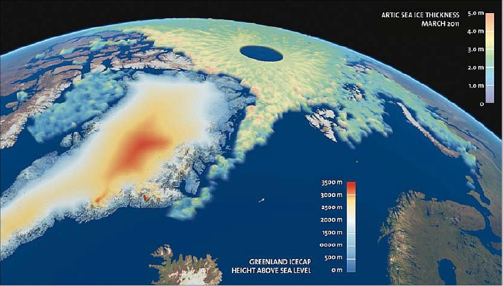
- February 2012: Ocean measurements from ESA’s CryoSat-2 mission are being exploited by the French space agency, CNES, to provide global ocean observation products in near-real time. Understanding sea-surface currents is important for marine industries and protecting ocean environments. 112)
- January 2012: Although the primary objective of CryoSat-2 was to measure the thickness of ice, fast data delivery was not initially intended. The CryoSat team has changed this to demonstrate that CryoSat-2 can deliver marine information in near-real time from most of its orbits around Earth. Up to now, this new product called 'fast delivery mode' has only been provided to organizations such as the US NOAA (National Ocean and Atmospheric Organization). This is about to change: marine information is expected to be available systematically to all users from February 2012 onwards. 113)
At NOAA’s LSA (Laboratory for Satellite Altimetry), the CryoSat-2 data are processed to estimate wind speed and wave height, which are then provided to forecasters at NOAA’s NCEPs (National Centers for Environmental Predication). LSA combines CryoSat-2 data with information from other organizations such as CNES of France, the ECMWF (European Centre for Medium-Range Weather Forecasts) and NASA. This processing takes a matter of only three days. NOAA delivers these data to ocean modelers and forecasters worldwide. For example, Australia’s Integrated Marine Observing System now uses CryoSat observations of sea level to monitor surface currents.
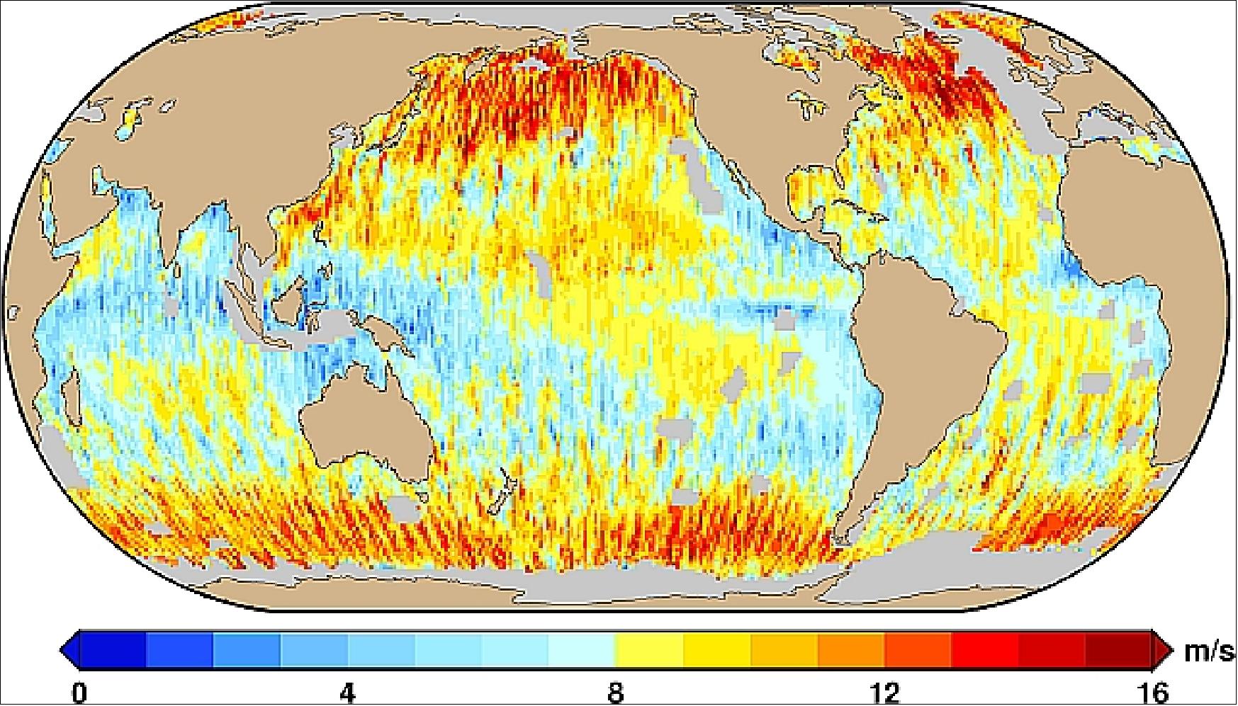
• Antarctic measurement campaign: In early December 2011, a team of Australian and German scientists from the University of Tasmania, the Australian Antarctic Division and the Alfred Wegner Institute (AWI, Bremerhaven) has just finished the first leg a remarkable measurement campaign. The campaign is being carried out in East Antarctica around Law Dome and the Totten Glacier. Law Dome is relatively stable but features steep surface slopes and Totten Glacier is changing rapidly – so both offer ideal locations for validating CryoSat-2 data. 114)
The campaign involves taking measurements from a Polar-6 aircraft. It carries the ASIRAS radar, which mimics CryoSat’s SIRAL. Ground-truth measurements are also collected for comparison. The skidoos drag GPS to map the height of the ice, which are later compared to the aircraft and satellite measurements. The skidoo team gathered ground measurement over about 250 km transects.
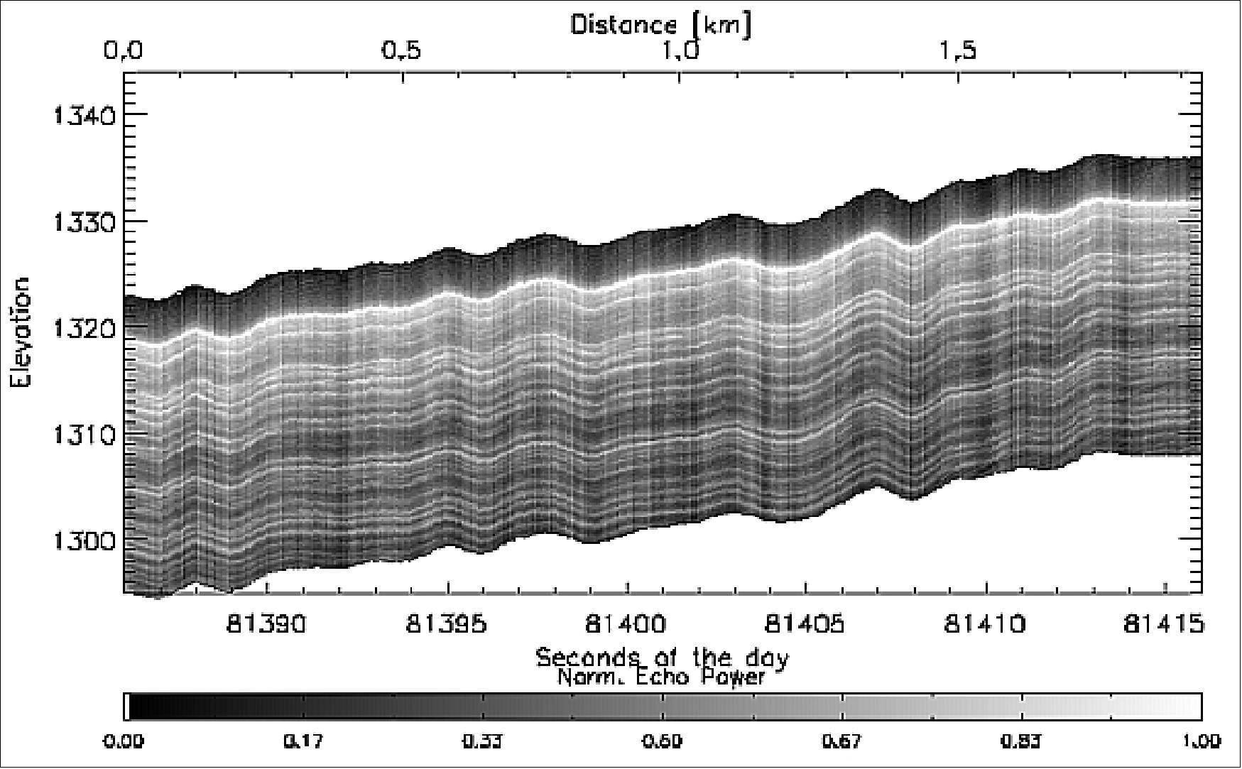
Legend to Figure 90: Strong layering as a result of seasonal changes in snow accumulation is clearly visible down to about 20 m. In combination with snow pit and firn-core data, scientists can determine the spatial variability of the accumulation rate (Ref. 114).
• The first map of sea-ice thickness from ESA’s CryoSat-2 mission was revealed at the Paris Air and Space Show on June 21, 2011. This new information is set to change our understanding of the complex relationship between ice and climate. CryoSat-2 has spent the last seven months delivering precise measurements to study changes in the thickness of Earth’s ice. 115)
CryoSat-2’s exceptionally detailed data have been used to generate this map of sea-ice thickness in the Arctic (Figure 91). Data from January and February of 2011 have been used to show the thickness of the ice as it approaches its annual maximum. Thanks to CryoSat-2’s orbit, ice thickness close to the North Pole can be seen for the first time.
CryoSat measures the height of the sea ice above the water line, known as the freeboard, to calculate the thickness. The data are exceptionally detailed and considerably better than the mission’s specification. They even show lineations in the central Arctic that reflect the ice’s response to wind stress.
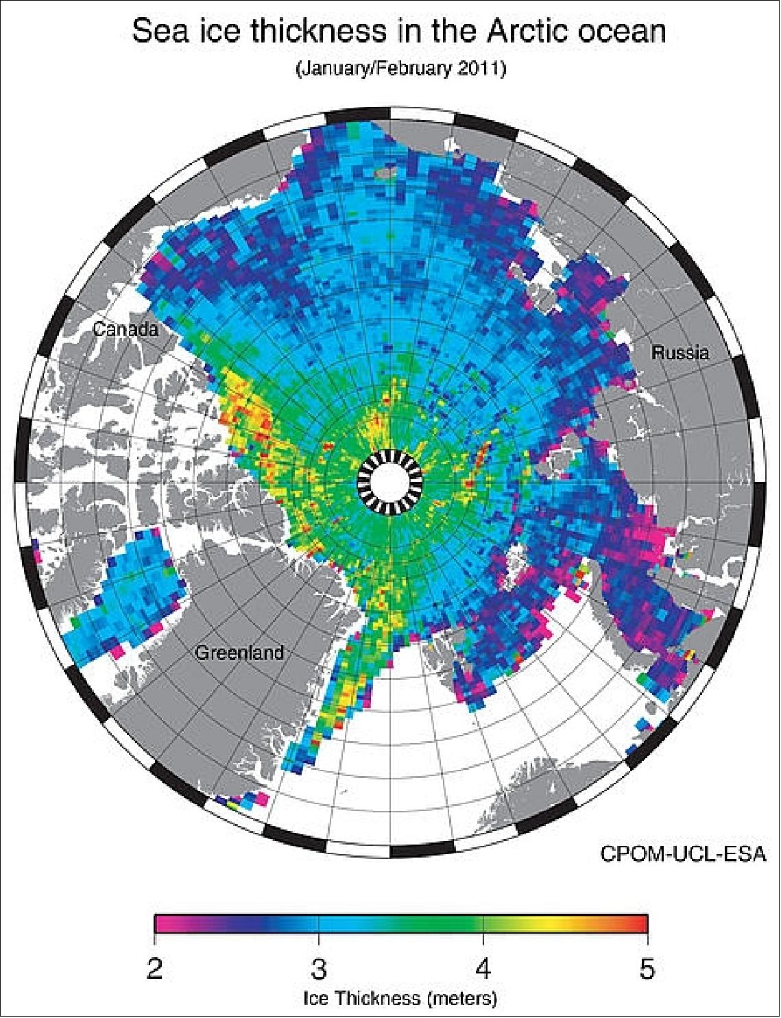
A new map of Antarctica has also been created showing the height of the ice sheet (Figure 92). This is more preliminary because more data are needed here to see what CryoSat-2 can do. Even so, the extra coverage that CryoSat-2 offers near the poles can be demonstrated: parts of Antarctica can now be seen for the first time from space.
In addition, detail of edges of the ice sheet where it meets the ocean can now closely be monitored thanks to CryoSat’s sophisticated radar techniques. This is important because this is where changes are occuring.
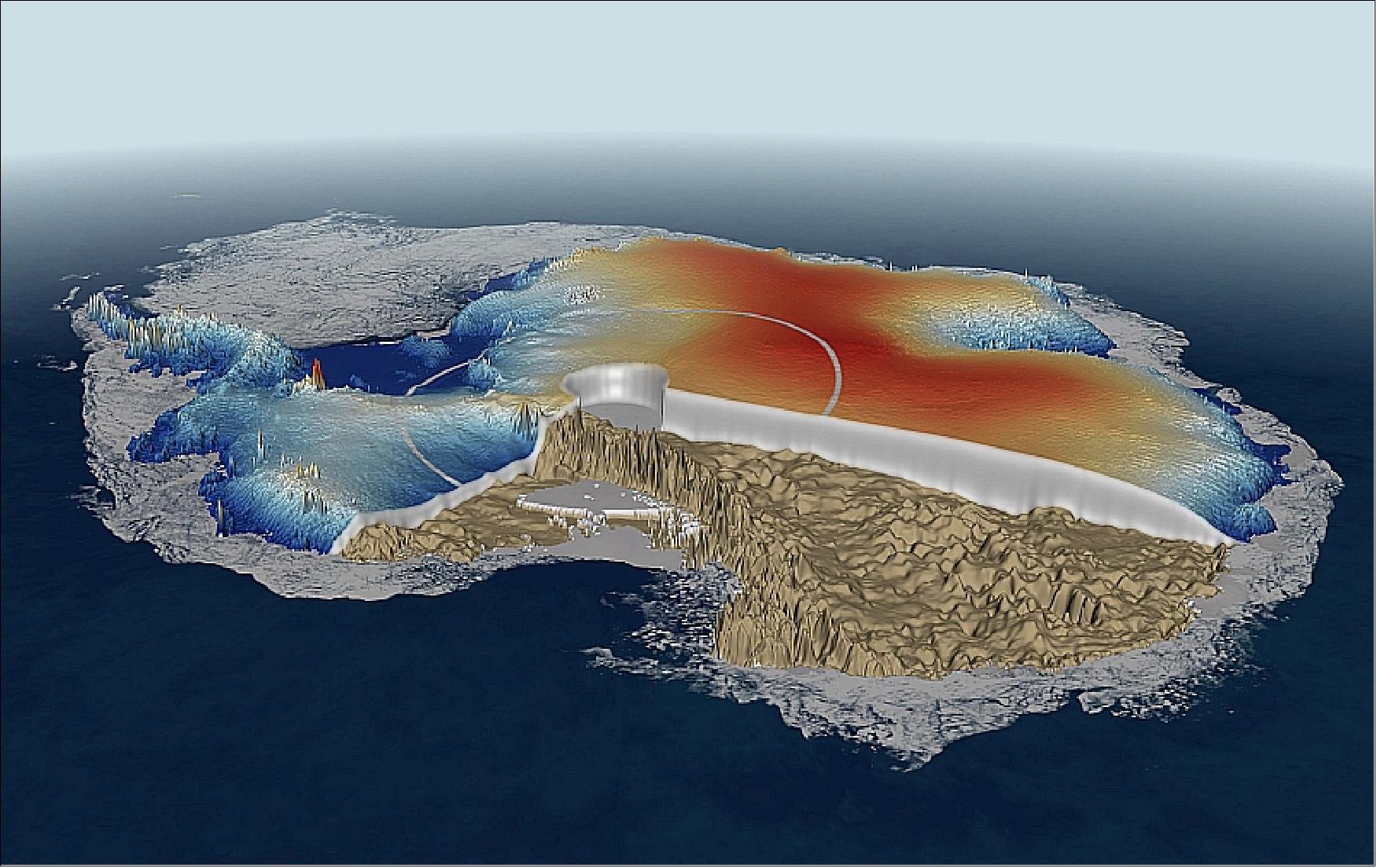
• A month-long common ESA/NASA Arctic campaign was conducted in the spring of 2011 in support of ESA's CryoSat mission. The one-month Arctic expedition is a major undertaking, with scientific teams from numerous organizations braving temperatures of –30ºC in central Greenland, Svalbard and the Fram Strait, Devon Island and offshore from Alert, Ellesmere Island, in northern Canada. 116)
To ensure that CryoSat is delivering accurate data, the scientists are gathering a wealth of ice and snow measurements on the ground and from the air. These in situ measurements will be compared with measurements delivered by CryoSat, thereby guaranteeing that the mission is delivering the best quality data possible. Data on changes in the thickness of ice floating in the polar oceans and in the vast ice sheets on land are vital in the quest to deepen our understanding of the delicate relationship between ice, climate change and sea-level rise.
In parallel, NASA is also in the Arctic, surveying the polar ice cover from the air for their IceBridge operation (see IceBridge below).
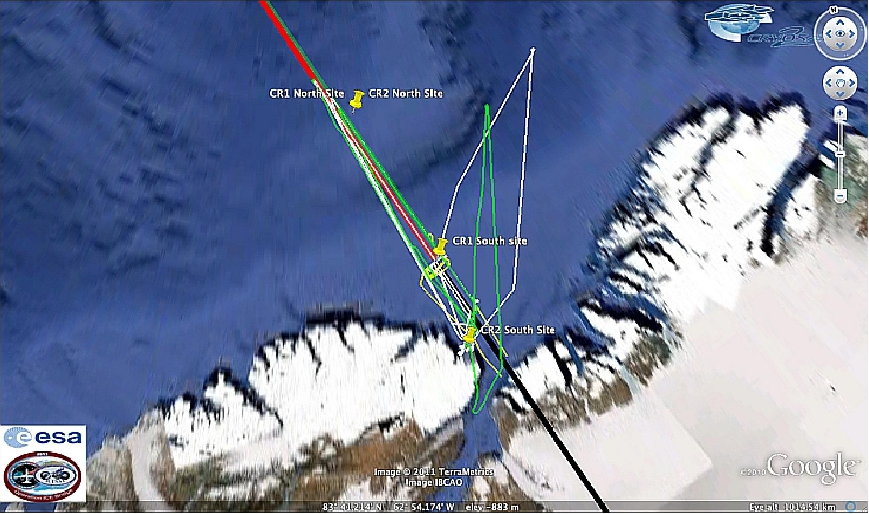
This involved coordinated ESA–NASA flight activities and orbital ground track of CryoSat on 17 April. In Figure 93, the straight red and black thick line indicates CryoSat's ground track and the color changes where the measurement mode switches to pass over the steep ice sheet margin. The dark green straight line shows the 15 April CryoSat track, with the yellow line indicating the NASA P-3 aircraft underflight. The white line shows the paths taken by the Twin Otter carrying the ASIRAS instrument and the green lines show the AWI aircraft carrying the electromagnetic sensor, which take measurements of the area for comparison.
NASA IceBridge campaigns: IceBridge, a six-year NASA mission, is the largest airborne survey of Earth's polar ice ever flown. It will yield an unprecedented three-dimensional view of Arctic and Antarctic ice sheets, ice shelves and sea ice. These flights will provide a yearly, multi-instrument look at the behavior of the rapidly changing features of the Greenland and Antarctic ice. IceBridge will use airborne instruments to map Arctic and Antarctic areas once a year. The first IceBridge flights were conducted in March/May 2009 over Greenland and in October/November 2009 over Antarctica. Other smaller airborne surveys around the world are also part of the IceBridge campaign. 117) 118)
- IceBridge has flown more than 200 hours during science flights with the P-3 during the 2011 Arctic deployment, and only one canceled flight day due to weather. On April 29, 2011, the P-3 flew a medium-priority mission over the catchment area of Petermann Gletscher that when combined with two other surveys will result in a 10-kilometer grid over the glacier’s entire catchment area. 119)
The ground measurements, multiple airborne measurements and the CryoSat-2 overpass will create a landmark dataset to shed light on fundamental issues in remotely sensing sea ice.
• On Feb. 1, 2011, ESA announced at the CryoSat Validation Workshop (Frascati, Italy, Feb. 1-3, 2011) the release of the CryoSat-2 ice data. This means that the international science community will have free and easy access to all of the measurements from CryoSat-2. This will amount to a unique dataset to determine the impact climate change is having on Earth's ice fields. 120)
• The CryoSat-2 mission was declared operational on Nov. 19, 2010. - The results of the intense commissioning phase were presented to more than 80 scientists and engineers from ESA, industry and universities at the CryoSat-2 Commissioning Results Review, held in Noordwijk, the Netherlands, on 22 October. 121) 122)
• The commissioning phase of the CryoSat-2 mission is expected to last for about 6 months.
• In mid-July 2010, the project is already releasing access data to about 150 scientists of around 40 research institutes (users outside the project team) as part of the calibration and validation procedure. The intent is to help ensure that these measurements meet the mission's exacting standards before the data are released to the wider scientific community later this year. 123)
• Taking advantage of NASA's 'Operation Ice Bridge' campaign in April 2010, measurements of Arctic sea ice have been made from an aircraft flying directly under CryoSat-2's orbital path. These measurements offer an early opportunity to check the quality of the newly launched CryoSat-2 satellite data over sea ice. The campaign uses a DC-8 aircraft carrying the ATM (Airborne Topographic Mapper) laser, which sends pulses of light in circular scans to the ground. The pulses reflected back to the aircraft are converted into elevation maps of the ice surface below.
Since the campaign is being carried out in the Arctic, ESA and NASA seized the opportunity to collaborate by timing one of the DC-8's flights to coincide with CryoSat-2 orbiting above. The NASA aircraft flew from Thule in northwestern Greenland over the Arctic Ocean on 20 April to pass directly under the satellite orbiting close to the North Pole. In parallel, ESA's European Spacecraft Operations Centre (ESOC) in Germany switched CryoSat-2's SIRAL from 'health monitoring mode' into its sea-ice measuring 'SAR mode'. 124)
- The first IceBridge underflight of CryoSat-2 took place on April 20, 2010 along a 670 km track over the Arctic Ocean. The flight was carried in using a NASA DC-8 as part of NASA’s Operation IceBridge and was designated Sea Ice 07. The aircraft intercepted the CryoSat-2 groundtrack near 87º latitude, 205º longitude approximately 10 minutes after the satellite passed over (13:33:06 GMT) as shown in Figure 94. The DC-8 followed the groundtrack westward at an altitude of 7000 m for about one hour, covering 670 km. The DC-8 carried the usual complement of IceBridge instrumentation, including the DMS (Digital Mapping System) camera, and two laser altimeters: 1.) the LVIS ( Land, Vegetation and Ice Sensor), usually flown at high altitudes, and 2.) the ATM (Airborne Topographic Mapper), usually flown at lower altitudes. 125)
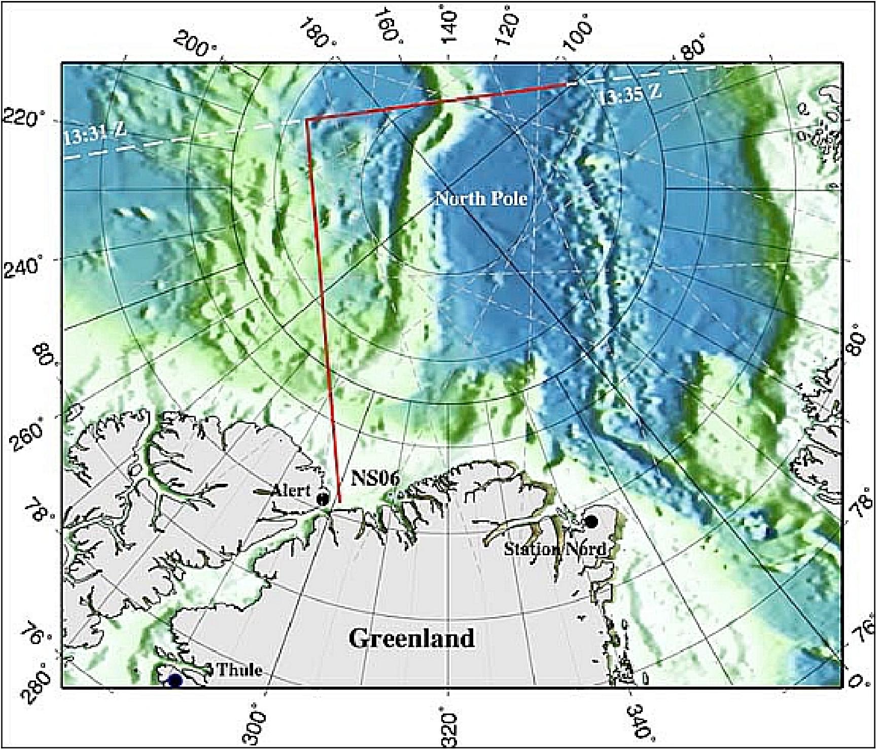
• On April 11, 2010, the LEOP (Launch and Early Orbit Phase) was formally ended. The spacecraft is in excellent condition. Later on April 11, SIRAL (Synthetic Aperture Interferometric Radar Altimeter) was switched on for the first time and started gathering the first radar echo data. 126)
• CryoSat-2 has delivered its first data just hours after ground controllers switched on the satellite's sophisticated radar instrument for the first time. CryoSat-2 was launched on 8 April and has been performing exceptionally well during these critical first few days in orbit.
Sensor Complement
SIRAL (SAR Interferometer Radar Altimeter)
SIRAL is the primary instrument of the mission, designed and developed for ESA by Thales Alenia Space (formerly Alcatel Alenia Space), France. SIRAL is of Poseidon-2 heritage flown on the Jason-1 mission. The objective is to observe ice sheet interiors, the ice sheet margins, for sea ice and other topography. 127)
The SIRAL-2 design is based on existing equipment, but with several major enhancements designed to overcome difficulties associated with measuring ice surfaces. It works by bouncing a radar pulse off the ground and studying the echoes from the Earth's surface. By knowing the position of the spacecraft - achieved with an onboard ranging instrument called DORIS (Doppler Orbitography and Radiopositioning Integrated by Satellite) - the signal return time will reveal the surface altitude. Correct antenna orientation is vital for this and is maintained using a trio of star trackers.
The design of SIRAL for the CryoSat-2 mission was made completely redundant. 128)
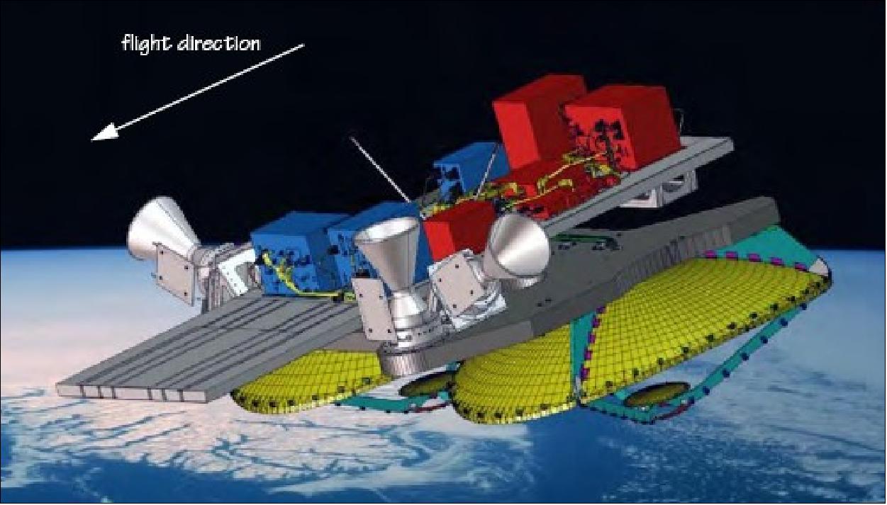
The SIRAL instrument design makes use of the DDA (Delay Doppler Altimeter) concept representing a new technology introduction into spaceborne altimetry and permitting that detailed views of irregular sloping edges of land ice, as well as non-homogenous ocean ice, can also be obtained. The new features of SIRAL have been demonstrated with the airborne D2P (Delay-Doppler Phase-monopulse Radar) of JHU/APL, first test flights were conducted in 2000 (for a DDA concept introduction see the last chapter of the description).
The SIRAL design features two receiving antennas forming an interferometer in the cross-track direction with a baseline of 1.2 m (support for SARIn mode). In addition, the return signal in along-track direction is processed to construct a synthetic aperture for enhanced ground resolution. The instrument is a Ku-band radar altimeter which uses the full-deramp range compression technique of conventional altimeters (conventional single frequency pulse-limited altimeter). However, it introduces two features that make it different from previous spaceborne altimeter implementations: 129) 130) 131) 132)
• The instrument has two parabolic antennas (including pulse-to-pulse phase coherence) and two receive chains, permitting an interferometric mode of operation (and interferometric signal processing).
• SIRAL operates at high PRF (Pulse Repetition Frequency), ensuring coherent along-track sampling for aperture synthesis (PRF>Doppler bandwidth). The distinguishing feature of SIRAL compared to conventional altimeter instruments (generally with pulse intervals of about 500 µs) is that it sends bursts of pulses separated by intervals of only 50 µs. Though the return echoes are correlated, the bursts are instead treated using “aperture synthesis” data processing techniques.

The instrument consists of three major subsystems, two of these are in discrete electronic boxes:
• DPU (Digital Processing Unit), it serves all digital altimeter functions, including the digital chirp generation, the full sequencing functions of the altimeter, and the receive and processing functions of the echo
• RFU (Radio Frequency Unit). It contains all analog IF and RF electronics and a solid-state power amplifier with an RF peak power of 25 W.
• The antenna subsystem consists of two Cassegrain antennas, mounted side-by-side and forming the interferometric cross-track. Both antennas are identical; one is used to transmit and receive, whereas the other antenna is used to receive echoes (bistatic configuration). The primary super-elliptic reflectors are about 1.1 m x 1.2 m in size. They are supported by a composite sandwich plate. A high thermoelastic stability is needed to meet the interferometric instrument performance.
Parameter | Value |
RF frequency | 13.575 GHz (single frequency Ku-band radar) |
Pulse bandwidth | 320 MHz, (40 MHz for tracking only in SARIn) |
PRF (Pulse Repetition Frequency) | 1.97 kHz in LRM, 17.8 kHz in SAR and in SARIn; coherent pulse transmission for Doppler processing |
Burst mode PRF | 1970 Hz in LRM, 85.7 Hz in SAR and 21.4 Hz in SARIn |
Pulse duration | 50 µs |
Timing | Regular PRF in LRM, burst mode in SAR/SARIn |
Samples/pulse | 128 in LRM and SAR, 512 in SARIn |
RF peak power | 25 W |
Antenna size | 2 reflectors 1.2 m x 1.1 m, side-by-side |
Antenna beamwidth (3 dB) | 1.08º (along-track) x 1.2º (cross-track) |
Antenna footprint | 15 km |
Range resolution | About 45 cm |
Along-track resolution | 250 m (SAR/SARIn) |
Data rate | 60 kbit/s for LRM, 12 Mbit/s in SAR, 2 x 12 Mbit/s in SARIn |
Instrument mass (with antennas) | 70 kg non-redundant |
Instrument power | 149 W |
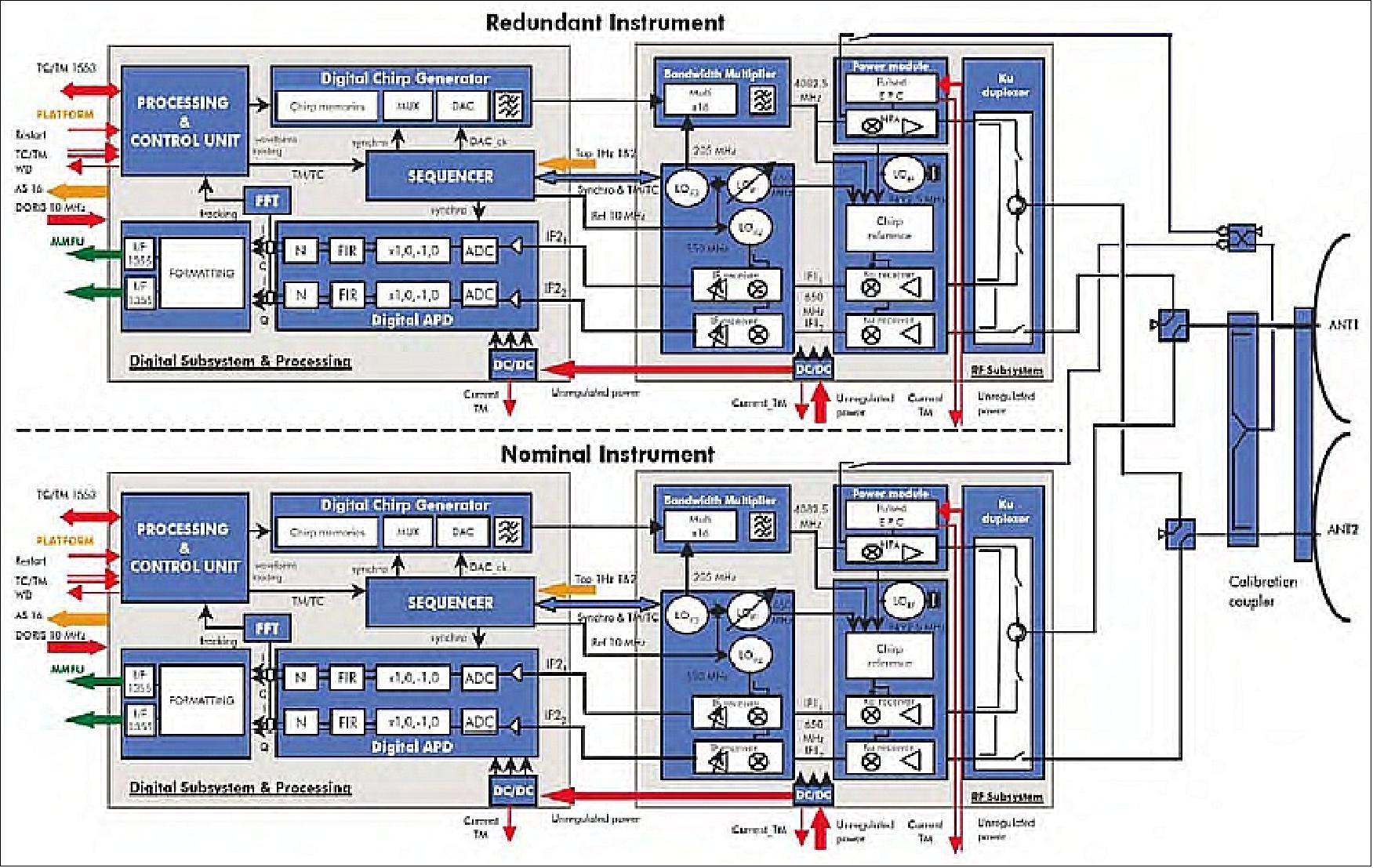
The science requirements demand of CryoSat to measure variations in ice thickness of perennial sea and land ice fields to the limit allowed by natural variability, on spatial scales varying over three orders of magnitude. The natural variability of sea and land ice depends on fluctuations in the supply of mass by the atmosphere and ocean, and snow and ice density. The precisions of the measurements are expressed in terms of cm of yearly ice equivalent thickness variations. These are:
• Arctic sea-ice: 1.6 cm/year vertical measurement accuracy at 105 km2 scale (equivalent to 300 km x 300 km cells). Temporal sampling: 1 month
• Land ice (small scale): 3.3 cm/year at 104 km2 (equivalent to 100 km x 100 km cells). Temporal sampling : 1 year
• Land-ice (large scale): 0.17 cm/year over 13.8 x 10⁶ km2 (about the area of Antarctica). Temporal sampling: 1 year.
Parameter | Coverage area (km2) | Science requirement | Measurement accuracy |
Arctic sea ice | 105 at or above 50º latitude | 3.5 cm/year | 1.6 cm/year |
Ice sheets | |||
Regional scale | 103 to 104 | 8.3 cm/year | 3.3 cm/year |
Antarctica | 106 | 0.76 cm/year | 0.17 cm/year |
The monitoring of the interferometric behavior of the receive chains is ensured by a dedicated interferometric calibration mode that can be used as an operational mode. An additional calibration mode permits the measurement of the amplitude/phase distortions of each receive chain. By using an internal frequency synthesizer, this measurement can be done for several frequencies inside the IF bandwidth. In addition, different gain settings can be used, which makes it possible to accurately determine the gain of the receiver. Either of the receive chain (chain 1 or 2) may be selected in LRM or in SAR support modes. This in-flight capability increases the knowledge of the instrument contribution on the echo measurement.
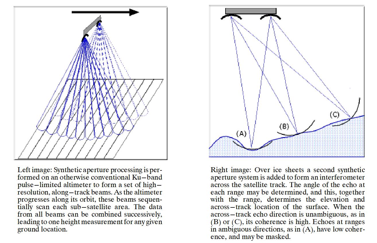
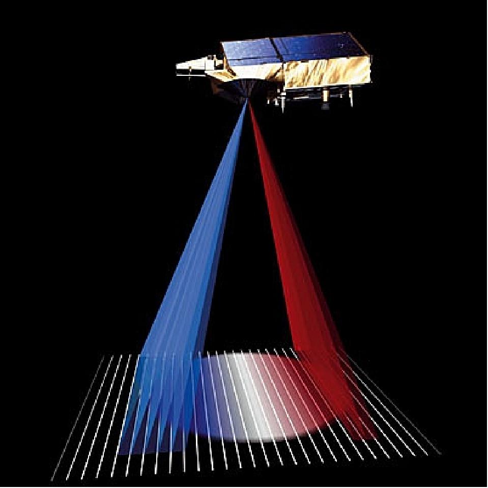
The chirp generator is composed of a digital pulse generation section, operating with a sampling rate of 160 MHz, followed by an analog multiplier section expanding the pulse bandwidth by a factor of 16, up to 350 MHz. This configuration ensures the pulse-to-pulse coherence required for the SAR modes. Parameters: chirp frequency = 4.08 GHz; bandwidth = 350 MHz; signal duration = 51 µs; SNR=30 dB.
The SSPA (Solid-State Power Amplifier) is composed of four parallel hybrid amplifiers in PHEMT technology. Parameters: frequency = 13.575 GHz; peak power >25 W; gain = 9 dB; amplitude ripple = 0.2 dB in 350 MHz; efficiency = 24%. - The FFT (Fast Fourier Transform) module, needed for the on-board tracking algorithm to estimate range and gain commands, makes use of the existing FFT module of POSEIDON 2.
SIRAL Operational Modes
SIRAL provides the following operational modes for different observational support types. The complex waveform data stream from the CryoSat altimeter requires a sophisticated processing scheme in particular for exploiting the synthetic aperture and interferometry techniques over ocean and ice surfaces.
1) LRM (Low Resolution Mode) operation support: LRM uses a single receive channel and low PRF for conventional pulse-limited operation for ice sheet interiors/open oceans. The transmitted pulse length and the transmitted bandwidth are set to the same value as that for Envisat in a similar mode (51 s, 320 MHz). The PRF is kept constant over the orbit at a value around 2 kHz to ensure the decorrelation of received echoes. The averaging for tracking and ground processing is performed after the FFT (Fast Fourier Transform).
The LRM mode is useful over surfaces where the topography is homogeneous, at least as large as the antenna footprint of about 15 km. The altimeter echoes have a predictable shape and the mean surface level of this area can be derived by an appropriate model.
2) SARM (Synthetic Aperture Radar Mode) support mode (also referred to as advanced SAR mode): SARM uses a single channel and a high PRF. Closed burst timing is employed to ensure a high along-track resolution. The PRF is chosen higher than the Doppler bandwidth over the half-power beamwidth to avoid aliasing in the ground processing of the data (the PRF is about 10 times higher than that of LRM to ensure coherence between the echoes of successive pulses). Bursts of 64 pulses at a PRF of 18.5 kHz with a burst repetition frequency of 85 Hz are transmitted.
In SARM, the resolution of the radar is improved in the along-track direction. This is achieved by exploiting the Doppler properties of the echoes as they cross the antenna beamwidth. The result is equivalent to decomposing the main antenna beam into a set of 64 narrower synthetic beams in the along-track direction. The footprints of the different sub-beams over a flat surface are adjacent rectangular areas, about 250 m wide in along-track and as large as the antenna's cross-track footprint (up to 15 km). Hence, a larger number of independent measurements are available over a given area; this property is used to enhance the accuracy of the measurements over sea ice. The echoes are transmitted to the ground segment in the time domain, prior to any averaging. Hence, the data rate in SARM is significantly higher than that for LRM.
3) SARIn (SAR Interferometric) support mode. The objective is to provide improved elevation estimates over variable topography. This mode is used mainly over ice sheet margins with high surface slopes. Both receive channels are operating simultaneously at high PRF to ensure the availability of a high cross-track resolution used for ice sheet margins and coastal areas (accurate determination of the arrival direction of the echoes in along-track and in cross-track). This is needed to derive the height of the surface from the range measurement of the radar. Narrow-band tracking pulses, transmitted in-between successive wide-band measurement bursts are used in this range-tracking concept to cope with abrupt height variations.
In the SARIn mode, the addition of the interferometric feature to the SAR further improves the echo localization capabilities, as the cross-track direction angle of the echoes can be determined. This is achieved by comparing the phase of one receive channel with respect to the other.
The innovative technical features of SIRAL are:
• The capability to operate in all measurement modes
• Digital chirp generation with pulse-to-pulse coherence for Doppler processing
• Solid State Power Amplifier (SSPA) in Ku-band with high performance (25 W),
• Dual antennas forming an interferometer, mounted on an optical bench together with star-tracker heads, ensuring the accurate knowledge and stability of the interferometric baseline orientation
• Two receive chains matched together with very low distortions.
The novel feature of SIRAL, as compared with conventional altimeters, is the capability to locate a resolution cell in the 3 dimensional space. The SIRAL concept is based on a Ku-band nadir-looking radar which can be operated in the conventional mode over oceans. Over terrain (ice or land) the “advanced SAR mode” uses Doppler filtering for the enhancement of the along-track resolution. A second antenna and receiving channel provides a second take of the scene which is used for surface height retrieval as it is usually done with SAR interferometry.
Parameter / Mode of Operation | LRM | SARM | SARIn |
Receive chain | 1 (left) | 1 (left) | 2 (left and right) |
Samples per echo | 128 | 128 | 512 |
Sample interval | 0.47 m | 0.47 m | 0.47 m |
Range window | 60 m | 60 m | 240 m |
Bandwidth | 350 MHz | 350 MHz | 350 MHz |
PRF | 1970 Hz | 17.8 kHz | 17.8 kHz |
Tx pulse length | 49 µs | 49 µs | 49 µs |
Useful echo length | 44.8 µs | 44.8 µs | 44.8 µs |
Burst length | N/A | 3.6 ms | 3.6 ms |
Pulses/burst | N/A | 64 | 64 |
Burst repetition interval | N/A | 11.7 ms | 46.7 ms |
Azimuth looks (46.7 ms) | 91 | 240 | 60 |
Tracking pulse bandwidth | 350 MHz | 350 MHz | 40 MHz |
Samples per tracking echo | 128 | 128 | 128 |
Size of tracking window | 60 m | 60 m | 480 m |
Averaged tracking pulses (46.7 ms) | 92 | 32 | 24 |
Data rate | 51 kbit/s | 11.3 Mbit/s | 2 x 11.3 Mbit/s |
Power consumption | 95.5 W | 127.5 W | 127.5 W |
Instrument mass (non redundant) | 62 kg | ||
Operations principle: Conventional radar altimeters send pulses with a long interval : about 500 µs. SIRAL sends a burst of pulses with an interval of only 50 µs between them. The returning echoes are thus correlated, and by treating the whole burst of pulses in one operation, the data processor can separate the echo into strips arranged across the track by exploiting the slight frequency shifts (caused by the Doppler effect) in the forward- and aft-looking parts of the beam. The strips laid down by successive bursts can therefore be superimposed on each other and averaged to reduce noise. This mode of operation is called the SARM (Synthetic Aperture Radar Mode). 133)
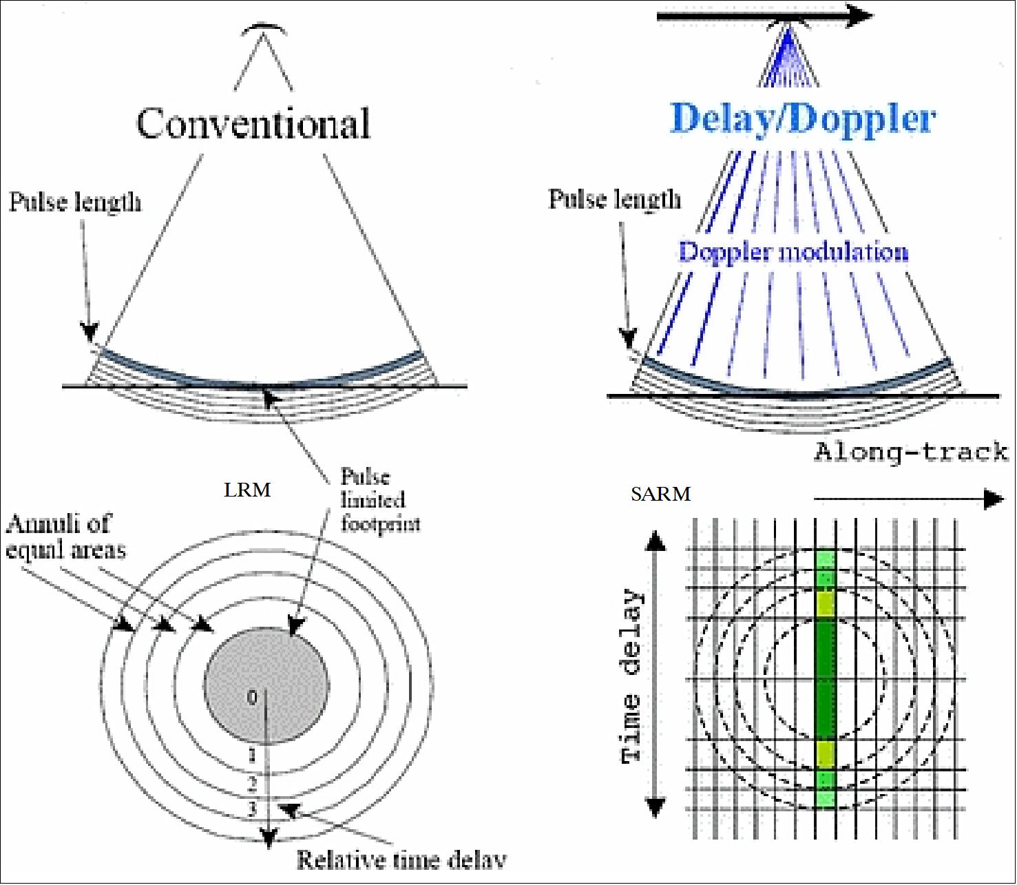
In interferometric mode (SARIn), a second receiving antenna is activated to measure the arrival angle. It enables to receive some radar echos coming from a point not directly located beneath the satellite. The difference in the path-length time of the radar echos is tiny between radar echos on the track and radar echoes out of the track. The measure of the angle between the baseline joining the antennas and the echo direction is essential and must be very accurate. The baseline orientation is so operated by three star trackers.
The Cryosat-2 mission is the first altimeter mission to operate the SARM (SAR mode), next to the LRM (Low Resolution Mode), in the SIRAL (SAT Interferometer Radar Altimeter) instrument.
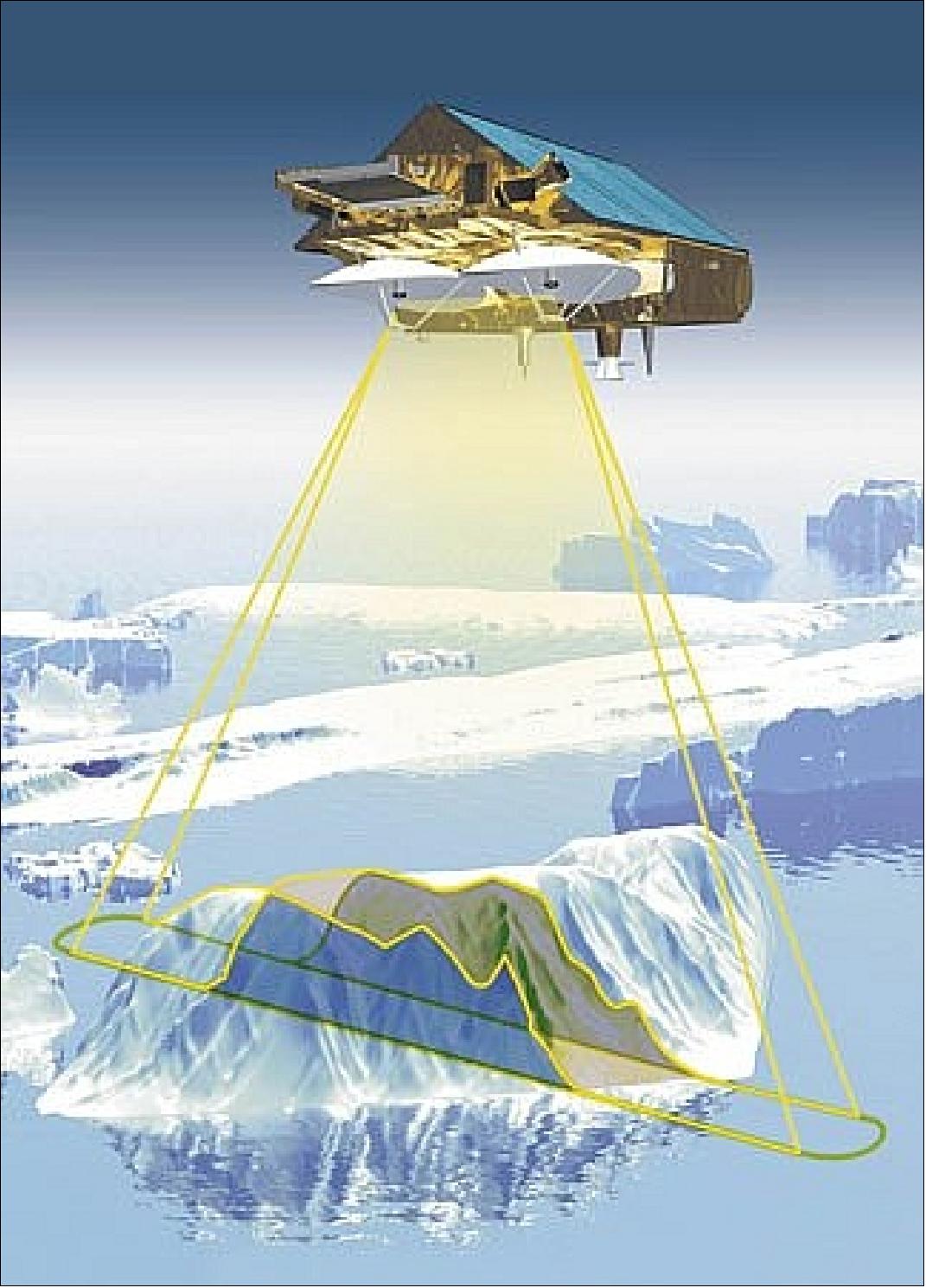
DORIS (Doppler Orbitography and Radiopositioning Integration by Satellite)
DORIS measures the Doppler frequency shifts of both VHF and S-Band signals transmitted by ground beacons. Its measurement accuracy is better than 0.5 mm/s in radial velocity allowing an absolute determination of the orbit position with an accuracy of 2-6 cm. DORIS is an uplink radio frequency tracking system based on the Doppler principle. The CNES instrument provides accurate measurements for a precise orbit determination. Knowledge of the orbit is essential for exploitation of the altimeter data and the overall performance. The onboard receiver measures the Doppler shift of uplink beacons in two frequencies (2.03625 GHz for Doppler measurement and 401.25 MHz for the ionospheric correction) which are transmitted continuously by the ground stations. One measurement is used to determine the radial velocity between spacecraft and beacon, the other to eliminate errors due to ionospheric propagation delays. The 401.25 MHz frequency is also used for measurements of time-tagging and auxiliary data transmission. The DORIS instrument comprises:
• A fixed omni-directional dual-frequency antenna
• A receiver performing the Doppler measurements every ten seconds. The nominal mode of operation is an autonomously programmed mode in which the receiver tracks the beacon signals according to information provided by the navigation software (DIODE) based on an on-board table of beacon data.
• An USO (Ultra Stable Oscillator) delivering the reference frequency with a stability of 5 x 10-13 over a period of 10 to 100 s.
The mass of DORIS is 15 kg (including the antenna of 160 mm diameter). The instrument requires 20 W of power, the data rate is 4 kbit/s.
The following DORIS services are used for CryoSat operations:
- Real-time orbit determination for spacecraft attitude and orbit control (on-board)
- Provision of a precise time reference based on TAI (International Atomic Time); in addition a precise 10 MHz reference signal is used (on-board)
- Provision of on-ground POD (Precise Orbit Determination) and ionospheric modelling.
The entire DORIS system comprises a network of more than 50 ground beacons, a number of receivers on several satellites in orbit and in development, and ground segment facilities. It is part of IDS (International DORIS Service), which also offers the possibility of precise localization of user-beacons.
LRR (Laser Retroreflector)
LRR is a passive optical device. The objective is to use LRR as an additional tool and backup for precise orbit determination with the aid of the international laser tracking network. LRR is accommodated in the nadir plate of the spacecraft, its FOV of ±57.6º is suitable for range measurements above 20º elevation angles at all azimuths from the ground. For any aspect angle the predicted rms target error is below 6 mm.
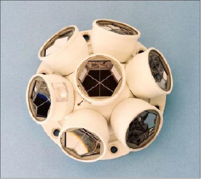
Prism material | Fused quartz |
Wavelength range | 310-1450 nm |
Free aperture diameter | 28.2 mm |
Reflective surface coating | Aluminum |
Reflective pattern width | 5-6 arcsec |
RMS target error | < 6 mm |
Introduction of the DDA (Delay Doppler Altimetry) technology into the SIRAL design
The concept of DDA, initially proposed by Keith Raney of JHU/APL (Johns Hopkins University/Applied Physics Laboratory), represents a new technology introduction with the potential to greatly increase the value of observations from satellite radar altimetry. The DDA scheme takes advantage of the Doppler shift of the pulse frequency in the along-track direction to allow for an increase in pulse repetition frequency and a subdivision of the illuminated area along-track into discrete Doppler bins to provide a dramatic improvement in efficiency and precision. 134) 135)
A conventional pulse-limited altimeter independently averages many radar pulses as the spacecraft moves along its track during the averaging time window and its illuminated area becomes defocused with increasing significant wave height. The relatively slow repetition of pulses and the impact of the waves limit the available resolution of the instrument.
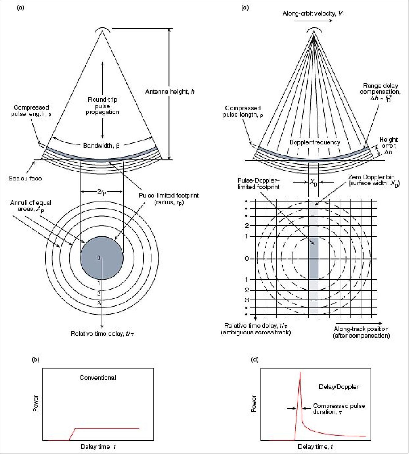
The DDA (Delay-Doppler Altimeter) differs from a conventional radar altimeter concept in that it exploits coherent processing of groups of transmitted pulses and the full Doppler bandwidth is exploited to make the most efficient use of the power reflected from Earth's surface. While the conventional altimeter technique is to measure the distance between the satellite and the mean ocean surface, the DDA method differs from those instruments in two ways: 136) 137) 138) 139)
- Pulse-to-pulse coherence and full Doppler processing to allow for measurement of the along-track position of the range measurement
- Use of two antennas and two receiver channels that allow for measurement of the across-track angle of the range measurement.
This is a significant improvement over conventional Doppler beam sharpening. To exploit this full bandwidth, the range variation that exists across the Doppler bins is removed as part of the data processing. The reflected pulses from a given area of the observed surface are integrated over the entire time that the target area is within the radar beamwidth. As a result, much more of the reflected energy is captured and a smaller transmitted power is required to obtain a given level of performance.
The DDA concept (Figure 103 b) retains the inherent advantages of a pulse-limited altimeter with its spherical wavefront always providing a nadir component, thus avoiding instrument nadir-pointing errors. In addition, the DDA exploits the faster pulse repetition frequency by binning the Doppler frequency shifts in the along-track direction. These bins appear as narrow strips orthogonal to the satellite ground track. As the DDA moves along its path, the leading edge Doppler bin illuminated during the first pulse becomes the second Doppler bin during the next pulse and receives a second “look” by the instrument. This process repeats as long as the bin remains within the DDA footprint. Each pulse defines a new leading edge Doppler bin, re-samples each bin within the footprint, and integrates the retrievals as the satellite moves along its track. Since each bin is sampled many times, the samples can be coherently processed and the higher pulse repetition frequency provides for a higher resolution footprint along-track that is independent of the significant wave height. For example, a 30 Hz altimeter pulse provides a signal integration length that results in widths of the Doppler bins as narrow as 250 m.
The DDA technology provides several advantages over conventional altimetry. The sea surface height precision available from this type of instrument is approximately twice that of existing sensors. Simulations of the associated signal processing concepts have produced 0.5 cm precision in a calm sea, with precision remaining better than 1.0 cm even in significant wave heights as great as 4 m. The DDA technique is much less sensitive to errors induced by ocean waves. For a calm sea, DDA and conventional altimetry experience comparable levels of random noise; however, as the waves grow, a conventional altimeter experiences a dramatic noise level increase. With the coherent processing of the DDA, only a slight increase in random noise with wave height is experienced. This makes the DDA particularly well suited for geodetic applications where the random error due to ocean waves is the dominant error source. Wind speed and wave height retrievals from the DDA have twice the precision of current sensors.
Another advantage of DDA is the ability to sample the coastal ocean where conventional altimeters experience signal contamination from land. As the spacecraft approaches or departs a coastline where the angle of intersection with the satellite ground track is nearly orthogonal, on board processing can identify individual Doppler bins close to the coast and continue to sample it as the satellite passes over the boundary.
From a system architecture perspective, the efficiency of the DDA provides for less transmitted power by the instrument and the potential for smaller and lighter spacecraft components - and thus a less costly mission - when compared to conventional altimeters with a similar design life.
There are also some data processing consequences with regard to SIRAL data which is based on the precise wavenumber domain approach. 140) 141) 142)
NOC Sea Level Anomaly (NOCSLA) Gridded Product
The new NOC Sea Level Anomaly (NOCSLA) gridded product is based on high-quality geophysical ocean products processed from SIRAL observations. This daily ¼° sea level anomaly product covers non-coastal oceans – from 60° north to 60° south – between January 2011 to October 2020.
To establish the scientific validity of NOCSLA, the product was compared against data delivered by a variety of space-borne sensors as part of a two-pronged verification process.
Firstly, NOCSLA was contrasted with observations from the international altimetry mission Jason-3, as well as with a sea level product produced by ESA’s Climate Change Initiative, and a sea surface height product produced by the Copernicus Climate Change Service (C3S).
Secondly, oceanic case studies were completed using NOCSLA and the results were compared with those from other data sources and models.
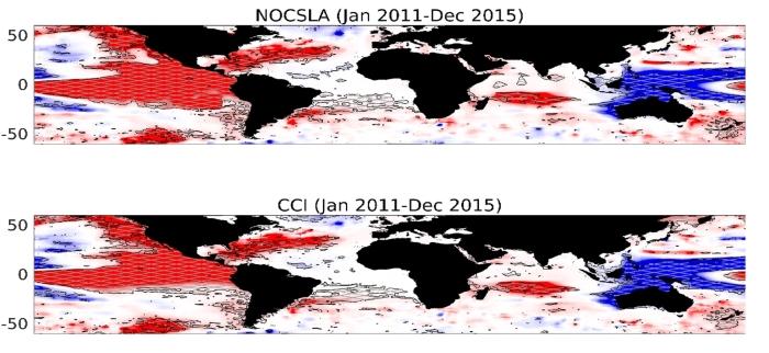
One study focused on assessing the product’s performance in observing events related to El Niño using NOAA’s ENSO (El Niño and the Southern Oscillation) index.
In another case study, NOCSLA data covering the Indian Ocean were used to investigate the occurrence of Rossby waves, also known as planetary waves, that form naturally in rotating fluids. These waves form as a result of Earth’s rotation. Rossby wave speeds determined by NOCSLA were in excellent agreement with a comparison dataset from ESA’s Climate Change Initiative.
Across both prongs of the verification process, NOCSLA outputs aligned well with ocean products from a variety of data sources, demonstrating the suitability of NOCSLA to enable a range of investigations into ocean processes.
Chris Banks, satellite oceanographer at NOC and lead author of the study, said: “Sea level anomaly products based on satellite data – such as the C3S product we employed in the NOCSLA validation – are already widely used.
“NOCSLA is unique because it is based on a single mission with a novel orbit, rather than a traditional repeat orbit every 10-30 days, and a long-term timeseries, creating a benefit for researchers and other data users.” 145)
Ground Segment
The CryoSat mission will be operated from ESA/ESOC, Darmstadt, Germany. The Kiruna ground station in Sweden functions as the prime command and data acquisition facility. The payload data segment (data processing, archiving and distribution) function is also located at the Kiruna station. The ground segment makes use of the existing infrastructure. All user interfaces are coordinated via ESA/ESRIN with dissemination of data from Kiruna.
An important aspect of the CryoSat-2 ground segment is that it had been designed for operations with a low level of manpower. Furthermore, remote operations and troubleshooting can be performed on all systems located in Kiruna.
The major elements of the ground segment are:
• RPF (Reference Planning Facility): responsible for the planning of the payload and the satellite resources verification.
• FOS (Flight Operations Segment): responsible for the telecommand scheduling, satellite command and control, and telemetry acquisition.
• PDS (Payload Data Segment): responsible of scientific data processing, archiving and distribution
• MF (Monitoring Facility): responsible for providing measures of the performance of the system, and in particular of the instruments.
• Complementary supporting ESA elements, shared with other missions:
- USF (User Services Facility)
- LTA (Long-Term Archive)
• Other elements outside ESA:
- DORIS control and processing centre (SSALTO) which provides precise orbits
- Auxiliary data providers (e.g. meteorological data)
- SLR (Satellite Laser Ranging) stations.
• User community, calibration, validation and retrieval.
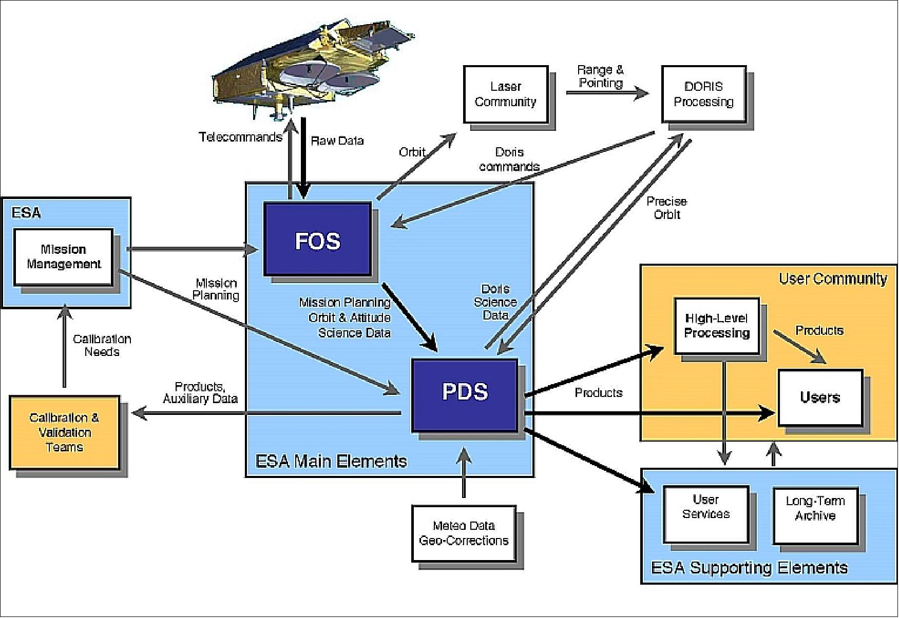
Permanent Calibration Station for Altimeters in Crete with Microwave Transponder
The Technical University of Crete (TUC) is installing a new permanent microwave transponder ground infrastructure on the Island of Crete, Greece, to serve as an alternative and independent technique for the calibration of, mainly, European altimetric missions. The facility was initially planned as a calibration site for the Sentinel-3 in the south west of Crete, Greece, using the developed transponder. However, this ground infrastructure, along with other permanent facilities in Crete, may also be used for the calibration of other Ku-band altimetric missions such Jason-2, Cryosat-2, etc. 143)
The idea for incorporating land based transponders was initially introduced in 2000. 144) A microwave transponder is an electronic equipment which receives the pulsed radar signal, transmitted by the altimeter of the over-passing satellite and actively amplifies and retransmits the signal towards the spacecraft, where it is recorded. The time delay of the signal is measured, from which the absolute range between the transponder and the satellite can be deduced. The main advantage of this technique, compared to the conventional sea-surface calibration, stands for the fact that no ocean dynamics errors are involved in satellite altimeter’s calibration.
However, in the past, only few transponders have been built and implemented for this reason. The ESA premises in Svalbard, Norway host a transponder developed by RAL, UK in 1987 that has been used mainly for the Cryosat-2 calibration. The Gavdos Island Cal/Val facility in Greece hosted the Austrian Academy of Sciences transponder and that transponder has been effectively used for the calibration of Envisat and Jason-2 missions. There has been another transponder placed in Rome, Italy which was used for the Envisat sigma-0 calibration.
TUC Transponder
In 2011, the Geodesy and Geomatics Engineering Laboratory at the Technical University of Crete in Greece developed a new Ku-band microwave transponder. The TUC transponder is mobile, allowing calibration at different locations but also modular for operating in other frequencies, provided that some parts are modified. It is capable of recording the incoming and outgoing signals, while it can be controlled and operated remotely. The transponder frequency has been selected to be compatible with past, current and future European as well as international altimetry missions that operate in this microwave range (i.e., Jason series, Cryosat-2, Sentinel-3). Additionally, it is equipped with a GPS (Global Navigation Satellite System) receiver and appropriate meteorological sensors to provide precise time-tagging, as well as the atmospheric delay corrections during transponder calibration. This is of importance for the accurate determination of the altimetric range because the atmosphere affects the altimetric measurements. Furthermore, this prototype transponder is the only microwave transponder that incorporates circularly polarized antennas. The latter, allows performing calibration experiments on different satellite missions at the same location, approaching from different directions, providing that the satellite ground track is in a range of 3-5 km away from the transponder location.
Parameter | Specification |
Frequency, bandwidth | 13.575 GHz, 350 MHz |
Gain stability | 0.5 dB |
Receiver noise figure | < 8 dB |
Internal electronics gain | 0.5 dB |
Antenna diameter | 90 cm |
The TUC transponder has been characterized for 4 months (March-July 2012) at the CPTR (Compact Payload Test Range) facilities in ESA/ESTEC, the Netherlands.
The transponder has already been used for the calibration of several Cryosat-2 passes (10-May, 8-June and 3-August 2013) over the SLR2 (Satellite Laser Ranging 2) site (35° 32.084' N, 24° 04.061' E) in North West Crete, Greece, and a clear response has been captured on the satellite’s data (Figure 105).
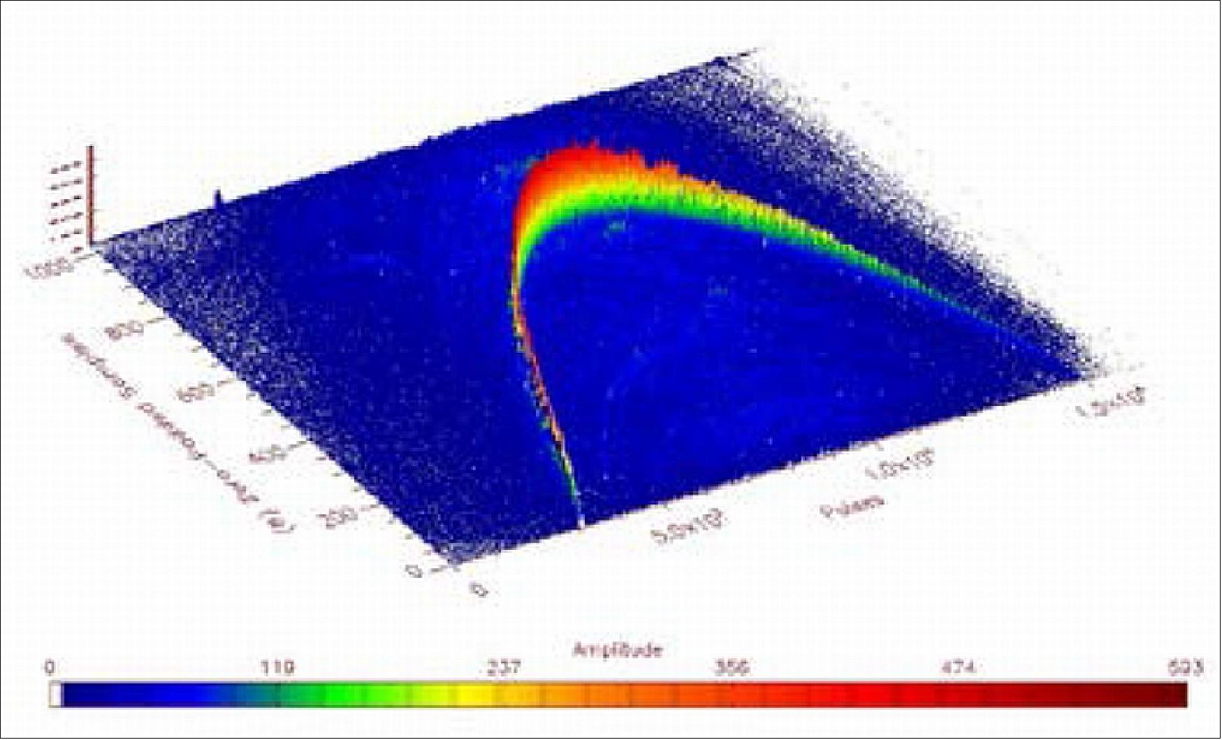
A TUC transponder site has been selected on Crete Island which represents a triple cross-over point between Sentinel-3A, -3B and Jason-2&3 (and also Jason-CS, as it will most likely fly over the same Jason-series tracks). This criterion was used to finally define and freeze the ground tracks for Sentinel-3 mission.
The CDN2 (35° 20.729' N, 23° 46.577'E) site is exactly under Jason, 100 m east of Sentinel-3A and 300 m west of the Sentinel-3B ground tracks. The CNES team will verify the satellite signal observed using Jason-2 around the CDN2 candidate.
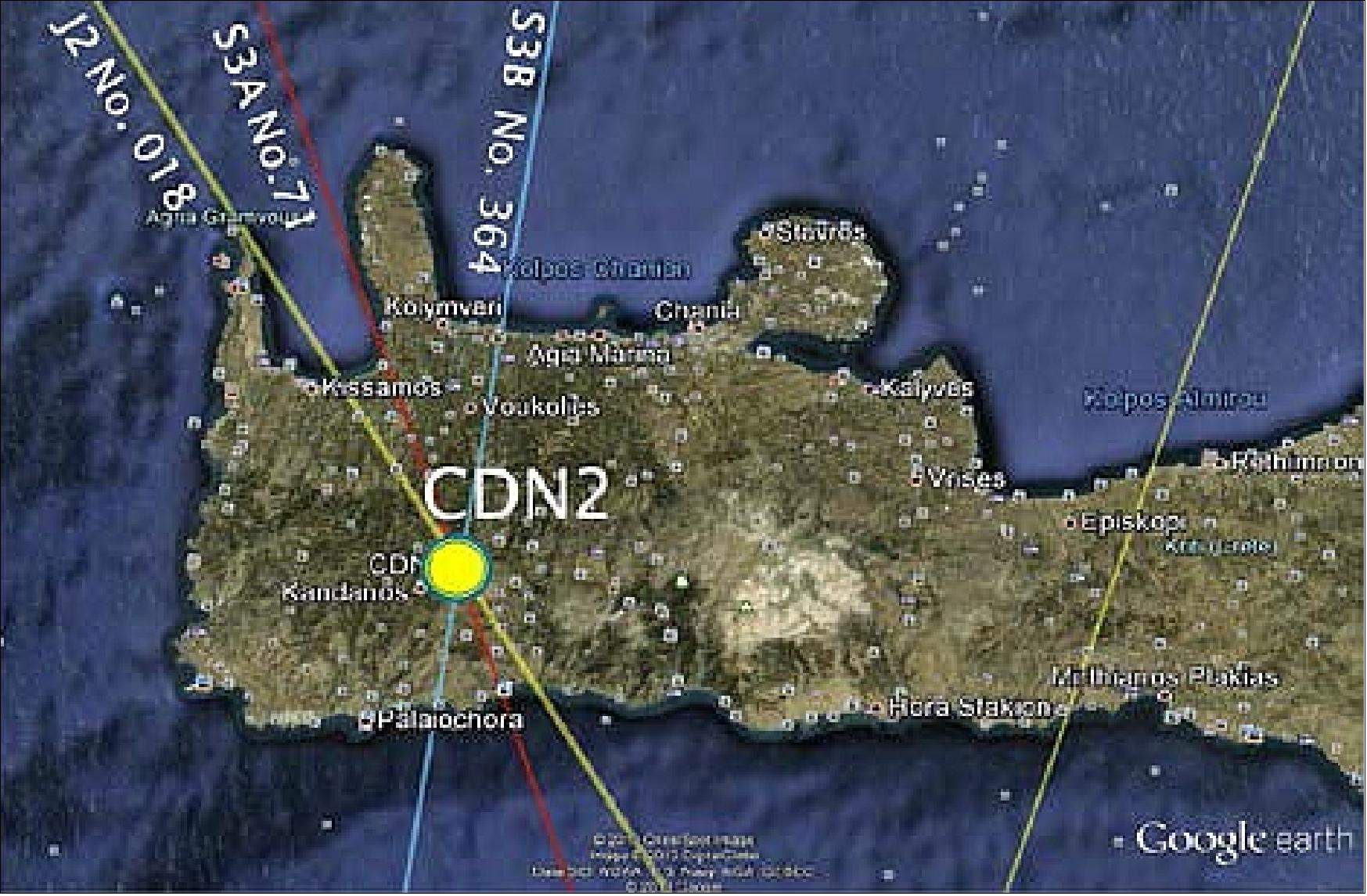
The instruments at the CDN2 site will be protected using either weather-proof boxes or a container with appropriate covers to avoid/reduce any satellite echoes by their metallic parts. Figure 107 illustrates an indicative spatial distribution of the necessary and ancillary instrumentation to be constructed at the CDN2 Sentinel-3 altimeter calibration site. Besides the instrumentation and infrastructure, the preparatory steps taken for the establishment of the CDN2 site involve also the development of appropriate software for data archival and transmission and for the determination of the transponder’s precise positioning.
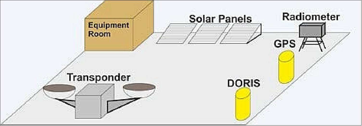
The Sentinel-3 altimeter calibration site is expected to be fully operational in early 2014, that is about one year prior to the Sentinel-3A launch. During this period, calibration campaigns for the Jason-2 and Cryosat-2 altimetry mission will be performed to test the transponder’s operational capabilities in real-field conditions. These campaigns will aim at: a) delivering altimeter calibration values for these satellites, b) getting familiarized with the remote operation procedures to be followed, and 3) identifying potential upgrades necessary for improving the transponder’s performance.
The transponder is to be upgraded, improved, and characterized before its final deployment and support for Sentinel-3A commissioning phase in 2015.
References
1) http://www.esa.int/SPECIALS/Cryosat/SEM7WFMVGJE_0.html
2) http://www.sciencedaily.com/releases/2007/03/070312111341.htm
3) http://www.esa.int/esaLP/SEMAD0Q11ZE_index_2.html
4) http://www.esa.int/esaLP/ESA0DL1VMOC_LPcryosat_0.html
5) Richard Francis, “ESA's Ice Mission, CryoSat: more important than ever,” ESA Bulletin Nr. 141, Feb. 2010, pp. 10-19
6) “Scientists and polar explorers brave the elements in support of CryoSat-2,” SpaceRef, April, 19, 2007, URL: http://www.spaceref.com/news/viewpr.html?pid=22417
7) Climate Change Students Help CryoSat-2 Arctic Campaign,” April 28, 2006, URL: http://www.esa.int/esaLP/SEM1OKOFGLE_index_0.html :
8) “Scientiists spend a white Christmas in Antarctica,” ESA, Dec. 22, 2008, URL: http://www.esa.int/esaCP/SEMP03TTGOF_index_0.html
9) “Scientists endure Arctic for last campaign prior to CryoSat-2 launch,” May 9, 2008, URL: http://www.esa.int/esaCP/SEMWGM2QGFF_index_0.html
10) “CryoSat Mission and Data Description,” Jan. 2, 2007, ESA/ESTEC, URL: http://esamultimedia.esa.int/docs/Cryosat/Mission_and_Data_Descrip.pdf
11) T. , N. Duske, S. Schulz, “The CryoSat AOCS - A cost-efficient design for small Earth Observation satellites,” 5th International ESA Conference on Guidance Navigation and Control Systems, Frascati, Italy, Oct. 22-25, 2002, ESA SP516
12) Stefano Pessina, Susanne Kasten-Coors, “In-Flight Characterization of CRYOSAT-2 Reaction Control System,” Proceedings of the 22nd International Symposium on Space Flight Dynamics (ISSFD), Feb. 28 - March 4, 2011, Sao Jose dos Campos, SP, Brazil, URL: http://www.issfd22.inpe.br/S7-Attitude.Dynamics.1-AD1/S7_P4_ISSFD22_PF_041.pdf
13) Peter Davidsen, Ole Mikkelsen, Henrik Lauritzen, “CryoSat-2 Therma star tracker in-orbit experiences,” Proceedings of the GNC 2011, 8th International ESA Conference on Guidance, Navigation & Control Systems, Carlsbad (Karlovy Vary), Czech Republic, June 5-10, 2011
14) P. Smith, S. Edwards, N. Solway, “CryoSat Cold Gas System and Component Development,” 40th AIAA/ASME/SAE/ASEE. Joint Propulsion Conference. July 11-14, 2004, Fort Lauderdale, FLA, USA
15) F. Marchese, D. Fornarelli, N. Mardle, S. Pessina, “CryoSat-2 AOCS LEOP and Commissioning,” Proceedings of the GNC 2011, 8th International ESA Conference on Guidance, Navigation & Control Systems, Carlsbad (Karlovy Vary), Czech Republic, June 5-10, 2011
16) D. Durrant, H. Crowle, J. Robertson, S. Dussy, “SiREUS - Status of the European MEMS Rate Sensor,” Proceedings of the 7th International ESA Conference on Guidance, Navigation & Control Systems, June 2-5, 2008, Tralee, County Kerry, Ireland
17) Dick Durrant, Stéphane Dussy, Brian Shackleton, Alan Malvern, “MEMS Rate Sensors in Space Becomes a Reality,” AIAA Guidance, Navigation and Control Conference and Exhibit, Aug. 20-23, 2007, Hilton Head, South Carolina, USA, AIAA 2007-6547
18) Benedict Olivier, “The SiREUS MEMS Rate Sensor Program,” Proceedings of the 59th IAC (International Astronautical Congress), Glasgow, Scotland, UK, Sept. 29 to Oct. 3, 2008, IAC–08-E5.1.09
19) “Successful launch for ESA’s CryoSat-2 ice satellite,” ESA, April 8, 2010, URL: http://www.esa.int/esaCP/SEMH5ZZNK7G_index_0.html
20) CryoSat-2 Launch Special,” ESA Bulletin No 142, May 2010, pp.62-63
21) Yuri N. Smagin, Vladimir A. Andreev, Alexander P. Svotin, “Details of Cryosat-2 Processing and Launch on DNEPR Launch Vehicle,” Proceedings of the Symposium on Small Satellite Systems and Services (4S), Funchal, Madeira, Portugal, May 31-June 4, 2010
22) “New launch date for CryoSat-2 confirmed,” ESA, March 19, 2010, URL: http://www.esa.int/SPECIALS/Cryosat/SEMIOT9KF6G_0.html
23) “February launch for ESA’s CryoSat ice mission,” ESA, Sept. 14, 2009, URL: http://www.esa.int/esaCP/SEMZT6W0EZF_index_0.html
24) ”CRYO2ICE over Antarctica: revealing further insight on changing ice,” ESA News, 12 July 2022, URL: https://earth.esa.int/eogateway/news/cryo2ice-over-antarctica-revealing-further-insight-on-changing-ice
25) ”Meltwater runoff from Greenland becoming more erratic,” ESA Applications, 3 November 2021, URL: https://www.esa.int/Applications/Observing_the_Earth/CryoSat/Meltwater_runoff_from_Greenland_becoming_more_erratic
26) Thomas Slater, Andrew Shepherd, Malcolm McMillan, Amber Leeson, Lin Gilbert, Alan Muir, Peter Kuipers Munneke, Brice Noël, Xavier Fettweis, Michiel van den Broeke & Kate Briggs, ”Increased variability in Greenland Ice Sheet runoff from satellite observations,” Nature Communications, Vol. 12, Article Number: 6069, Published: 1 November 2021, https://doi.org/10.1038/s41467-021-26229-4, URL: https://www.nature.com/articles/s41467-021-26229-4.pdf
27) ”Arctic coastal sea ice thinning twice as fast than thought,” ESA Applications / Observing the Earth / CryoSat, 10 June 2021, URL: https://www.esa.int/Applications/Observing_the_Earth/CryoSat/Arctic_coastal_sea_ice_thinning_twice_as_fast_than_thought
28) Robbie D. C. Mallett, Julienne C. Stroeve, Michel Tsamados, Jack C. Landy, Rosemary Willatt, Vishnu Nandan, and Glen E. Liston, ”Faster decline and higher variability in the sea ice thickness of the marginal Arctic seas when accounting for dynamic snow cover,” The Cryosphere, Vol. 15, pp: 2429-2450, Published: 04 June 2021, https://doi.org/10.5194/tc-15-2429-2021
29) ”CryoSat reveals ice loss from glaciers in Alaska and Asia,” ESA Applications, 01 June 2021, URL: http://www.esa.int/Applications/Observing_the_Earth/CryoSat/CryoSat_reveals_ice_loss_from_glaciers_in_Alaska_and_Asia
30) Livia Jakob, Noel Gourmelen, Martin Ewart, and Stephen Plummer, ”Spatially and temporally resolved ice loss in High Mountain Asia and the Gulf of Alaska observed by CryoSat-2 swath altimetry between 2010 and 2019,” The Cryosphere, Volume 15, pp: 1845–1862, 2021, Published: 14 April 2021, https://doi.org/10.5194/tc-15-1845-2021, , URL: https://tc.copernicus.org/articles/15/1845/2021/tc-15-1845-2021.pdf
31) ”Arctic sea ice succumbs to Atlantification,” ESA Applications, 21 May 2021, URL: https://www.esa.int/Applications/Observing_the_Earth/CryoSat/Arctic_sea_ice_succumbs_to_Atlantification
32) ”Winners presented with ESA-EGU Excellence award,” ESA Applications, 19 April 2021, URL: https://www.esa.int/Applications/Observing_the_Earth/Winners_presented_with_ESA-EGU_Excellence_award
33) ”CryoSat reveals surprising ebb and flow of subglacial lakes,” ESA Applications, 14 December 2020, URL: http://www.esa.int/Applications/Observing_the_Earth/CryoSat/CryoSat_reveals_surprising_ebb_and_flow_of_subglacial_lakes
34) ”Places in Antarctica named in honor of ice scientists,” ESA / Applications / Observing the Earth / CryoSat, 09 December 2020, URL: https://www.esa.int/Applications/Observing_the_Earth/CryoSat/Places_in_Antarctica_named_in_honour_of_ice_scientists
35) ”CryoSat taken to new heights for ice science,” ESA Applications, 03 August 2020, URL: https://www.esa.int/Applications/Observing_the_Earth/CryoSat/CryoSat_taken_to_new_heights_for_ice_science
36) ”CryoSat still cool at 10,” ESA / Applications / Observing the Earth / CryoSat, 8 April 2020, URL: http://www.esa.int/Applications/Observing_the_Earth/CryoSat/CryoSat_still_cool_at_10
37) ”CryoSat sheds new light on Antarctica’s biggest glacier,” ESA / Applications / Observing the Earth / CryoSat, 27 January 2020, URL: http://www.esa.int/Applications/Observing_the_Earth/CryoSat/CryoSat_sheds_new_light_on_Antarctica_s_biggest_glacier
38) ”CryoSat maps ice shelf on the move,” ESA / Applications / Observing the Earth / CryoSat, 13 December 2019, URL: http://www.esa.int/Applications/Observing_the_Earth/CryoSat/CryoSat_maps_ice_shelf_on_the_move
39) Jan Wuite, Thomas Nagler, Noel Gourmelen, Maria Jose Escorihuela, Anna E. Hogg and Mark R. Drinkwater, ”Sub-Annual Calving Front Migration, Area Change and Calving Rates from Swath Mode CryoSat-2 Altimetry, on Filchner-Ronne Ice Shelf, Antarctica,” Remote Sensing, Published 23 November 2019, Volume 11, Issue 23, 2761, https://doi.org/10.3390/rs11232761
40) ”CryoSat conquers ice on Arctic lakes,” ESA, 5 August 2019, URL: http://www.esa.int/Our_Activities/Observing_the_Earth/CryoSat/CryoSat_conquers_ice_on_Arctic_lakes
41) Justin F. Beckers, J. Alec Casey, Christian Haas, ”Retrievals of Lake Ice Thickness From Great Slave Lake and Great Bear Lake Using CryoSat-2,” IEEE Transactions on Geoscience and Remote Sensing, Volume 55, Issue: 7, July 2017, URL: https://web.archive.org/web/20221218192024/http://ieeexplore.ieee.org/document/7891554/
42) ”Expanding our knowledge of Arctic Ocean bathymetry,” ESA, 24 July 2019, URL: http://m.esa.int/Our_Activities/Observing_the_Earth/CryoSat/Expanding_our_knowledge_of_Arctic_Ocean_bathymetry
43) Adili Abulaitijiang, Ole Baltazar Andersen, David Sandwell, ”Improved Arctic Ocean Bathymetry derived from DTU17 Gravity model,” AGU 100 (Advancing Earth and Space Science), First published: 08 July 2019, https://doi.org/10.1029/2018EA000502
44) ”Modelling tides in the Arctic Ocean,” ESA, 11 July 2019, URL: http://www.esa.int/Our_Activities/Observing_the_Earth/CryoSat/Modelling_tides_in_the_Arctic_Ocean
45) M. Cancet, O. B. Andersen, F. Lyard, D. Cotton, J. Benveniste, ”Arctide2017, a high-resolution regional tidal model in the Arctic Ocean,” Advances in Space Research, Volume 62, Issue 6, 15 September 2018, Pages 1324-1343, URL: https://tinyurl.com/y2axpw8c
46) ”Antarctica detailed in 3D,” ESA, 14 May 2019, URL: http://www.esa.int/spaceinimages/Images/2019/05/Antarctica_detailed_in_3D
47) N. Gourmelen,M. J. Escorihuela, A. Shepherd, L. Foresta, A. Muir, A. Garcia-Mondéjar, M. Roca, S. G. Baker, M. R. Drinkwater, ”CryoSat-2 swath interferometric altimetry for mapping ice elevation and elevation change,” Advances in Space Research, Volume 62, Issue 6, 15 September 2018, Pages 1226-1242, https://doi.org/10.1016/j.asr.2017.11.014, URL: https://tinyurl.com/y63k74v2
48) ”US government shutdown effects on CryoSat geophysical corrections and parameters,” ESA, 23 January 2019, URL: https://web.archive.org/web/20191227133848/https://earth.esa.int/web/guest/missions/esa-operational-eo-missions/cryosat/news/-/article/us-government-shutdown-effects-on-cryosat-geophysical-corrections-and-parameters
49) T. Parrinello, A. Shepherd, J. Bouffard, S. Badessi, T. Casal, M. Davidson, M. Fornari, E. Maestroni, M. Scagliola, ”CryoSat: ESA’s ice mission – Eight years in space,” Advances in Space Research, Vol. 62, Issue 6, 15 September 2018, pp: 1178–1190, https://doi.org/10.1016/j.asr.2018.04.014, Published by Elsevier Ltd.,URL: http://tinyurl.com/y2uzf5xr
50) ”New view of Antarctica in 3D,” ESA, 11 May 2018, URL: http://m.esa.int/Our_Activities/Observing_the_Earth/CryoSat/New_view_of_Antarctica_in_3D
51) ”CryoSat reveals retreat of Patagonian glaciers,” ESA, 2 May 2018, URL: http://m.esa.int/Our_Activities/Observing_the_Earth/CryoSat/CryoSat_reveals_retreat_of_Patagonian_glaciers
52) L. Foresta, N. Gourmelen, F. Weissgerber, P. Nienow, J. J. Williams, A. Shepherd, M. R. Drinkwater, S. Plummer, ”Heterogeneous and rapid ice loss over the Patagonian Ice Fields revealed by CryoSat-2 swath radar altimetry,” Remote Sensing of Environment, Available online 20 April 2018, https://doi.org/10.1016/j.rse.2018.03.041
53) ”Antarctica loses grip,” ESA, 3 April 2018, URL: http://m.esa.int/Our_Activities/Observing_the_Earth/CryoSat/Antarctica_loses_grip
54) Hannes Konrad, Andrew Shepherd, Lin Gilbert, Anna E. Hogg, Malcolm McMillan, Alan Muir, Thomas Slater, ”Net retreat of Antarctic glacier grounding lines,” Nature Geoscience, 2018, URL: https://www.nature.com/articles/s41561-018-0082-z.epdf?author_access_token=HCt_-ggOqYI1iPWrsR-BINRgN0jAjWel9jnR3ZoTv0PwzmpCvh7bKPjXpWeaTWIEiwEEdPz4GfJiBeHy6NOuuZ3WoFwUDLq8F36txXpSfoAD5yEjM0CMICYGZHTlKXPqt6QGyeIMDNsHH0PlKmlOjQ%3D%3D
55) ”Shifting grounding lines,” ESA, 3 April 2018, URL: http://m.esa.int/spaceinimages/Images/2018/04/Shifting_grounding_lines
56) ”Effect of grounding line on surface,” ESA, 3 April 2018, URL: http://m.esa.int/spaceinimages/Images/2018/04/Effect_of_grounding_line_on_surface
57) ”Secrets of hidden ice canyons revealed,” ESA, 11 Oct. 2017, URL: http://m.esa.int/Our_Activities/Observing_the_Earth/CryoSat/Secrets_of_hidden_ice_canyons_revealed
58) ”Giant iceberg in the making,”ESA, July 5, 2017, URL: http://m.esa.int/Our_Activities/Observing_the_Earth/CryoSat/Giant_iceberg_in_the_making
59) ”Historical iceberg tracks,” ESA,5 July 2017, URL: http://m.esa.int/spaceinimages/Images/2002/07/Historical_iceberg_tracks
60) ”CryoSat reveals Antarctica in 3D,” ESA, March 24, 2017, URL: http://m.esa.int/Our_Activities/Observing_the_Earth/CryoSat/CryoSat_reveals_Antarctica_in_3D
61) ”To the Arctic for CryoSat and beyond,” ESA, March 20, 2017, URL: http://m.esa.int/Our_Activities/Observing_the_Earth/CryoSat/To_the_Arctic_for_CryoSat_and_beyond
62) ”Two frequencies on one plane,” ESA, March 20, 2017, URL: http://m.esa.int/spaceinimages/Images/2017/03/Two_frequencies_on_one_plane
63) ”CryoSat reveals lake outbursts beneath Antarctic ice,” ESA, Feb. 8, 2017, URL: http://m.esa.int/Our_Activities/Observing_the_Earth/CryoSat/CryoSat_reveals_lake_outbursts_beneath_Antarctic_ice
64) Benjamin E. Smith, Noel Gourmelen, Alexander Huth, Ian Joughin, ”Connected subglacial lake drainage beneath Thwaites Glacier, West Antarctica,” The Cryosphere, Vol. 11, pp: 451-467, doi:10.5194/tc-11-451-2017, published on Feb. 8, 2017, URL: http://www.the-cryosphere.net/11/451/2017/tc-11-451-2017.pdf
65) ”Glacier speed West Antarctica,” ESA, released Feb. 8, 2017, URL: http://m.esa.int/spaceinimages/Images/2017/02/Glacier_speed_West_Antarctica
66) ”Satellite cousins have ice covered,” ESA, Dec. 16, 2016, URL: http://m.esa.int/Our_Activities/Observing_the_Earth/SMOS/Satellite_cousins_have_ice_covered
67) ”Arctic freeze slows down,” ESA, Nov. 30, 2016, URL: http://m.esa.int/Our_Activities/Observing_the_Earth/CryoSat/Arctic_freeze_slows_down
68) ”CryoSat sets new standard for measuring sea levels,” ESA, July 26, 2016, URL: http://m.esa.int/Our_Activities/Observing_the_Earth/CryoSat/CryoSat_sets_new_standard_for_measuring_sea_levels
69) ESA SP-1333 ESA's Report to the 41th COSPAR meeting, 21 July 2016, 'Status of the CryoSat mission,' pp: 24-25, URL: http://esamultimedia.esa.int/multimedia/publications/SP-1333/SP-1333.pdf
70) ”The Arctic is facing a decline in sea ice that might equal the negative record of 2012 — Data collected by the CryoSat-2 satellite reveal large amounts of thin ice that are unlikely to survive the summer,” AWI Press Release, April 21, 2016, URL: http://www.awi.de/nc/en/about-us/service/press/press-release/der-arktis-droht-ein-meereisverlust-wie-im-negativrekordjahr-2012.html
71) EGU General Assembly 2016, Vienna Austria, April 17-22, 2016
72) Jonathan Amos, ”Call for dedicated polar Sentinel satellite,” BBC News, March 24, 2016, URL: http://www.bbc.com/news/science-environment-35886817
73) ”Ice matters,” ESA's Climate Change Initiative, Dec. 11, 2015, URL: http://www.esa.int/Our_Activities/Space_for_climate/Ice_matters
74) “Cool summer boosts Arctic ice,” ESA, July 20, 2015, URL: http://www.esa.int/Our_Activities/Observing_the_Earth/CryoSat/Cool_summer_boosts_Arctic_ice
75) Rachel L. Tilling, Andy Ridout, Andrew Shepherd, Duncan J. Wingham, “Increased Arctic sea ice volume after anomalously low melting in 2013,” Nature Geoscience, (2015) doi:10.1038/ngeo2489, published online July 20, 2015
76) “CryoSat detects sudden ice loss in Southern Antarctic Peninsula,” ESA, May 22, 2015, URL: http://www.esa.int/Our_Activities/Observing_the_Earth/CryoSat/CryoSat_detects_sudden_ice_loss_in_Southern_Antarctic_Peninsula
77) “Fast access to CryoSat’s Arctic ice measurements now available,” ESA, April 17, 2015, URL: http://www.esa.int/Our_Activities/Observing_the_Earth/CryoSat/Fast_access_to_CryoSat_s_Arctic_ice_measurements_now_available
78) “CryoSat Operational Polar Monitoring,” URL: https://web.archive.org/web/20150420104755/http://www.cpom.ucl.ac.uk/csopr/index.html
79) “Ice ventures yield results for CryoSat-2,” ESA, March 18, 2015, URL: http://www.esa.int/Our_Activities/Observing_the_Earth/CryoSat/Ice_venturers_yield_results_for_CryoSat
80) Satellites catch Austafonna shedding ice,” ESA, Jan. 23, 2015, URL: http://www.esa.int/Our_Activities/Observing_the_Earth/Satellites_catch_Austfonna_shedding_ice
81) Malcolm McMillan, Andrew Shepherd, Noel Gourmelen, Amaury Dehecq, Amber Leeson, Andrew Ridout, Thomas Flament, Anna Hogg, Lin Gilbert, Toby Benham, Michiel van den Broeke, Julian A. Dowdeswell, Xavier Fettweis, Brice Noël, Tazio Strozzi, “Rapid dynamic activation of a marine-based Arctic ice cap,” Geophysical Research Letters, Volume 41, Issue 24, pp: 8902–8909, 28 December 2014, DOI: 10.1002/2014GL062255
82) CryoSat-2 extends its reach on the Arctic,” ESA, Dec. 15, 2014, URL: http://www.esa.int/Our_Activities/Observing_the_Earth/CryoSat/CryoSat_extends_its_reach_on_the_Arctic
83) “CryoSat,” ESA Bulletin, No 160, November 2014, p. 73
84) “CryoSat unveils secrets of the deep,” ESA, Oct. 3, 2014, URL: http://www.esa.int/Our_Activities/Observing_the_Earth/CryoSat/CryoSat_unveils_secrets_of_the_deep
85) David T. Sandwell, R. Dietmar Müller, Walter H. F. Smith, Emmanuel Garcia, Richard Francis, “New global marine gravity model from CryoSat-2 and Jason-1 reveals buried tectonic structure,” Science, October 3, 2014, Vol. 346 No 6205, pp: 65-67, DOI: 10.1126/science.1258213
86) “Greenland ice-sheet height,” ESA, Aug. 20, 2014, URL: http://www.esa.int/Our_Activities/Observing_the_Earth/CryoSat/Ice_sheet_highs_lows_and_loss
87) Veit Helm, A. Humbert, H. Miller, “Elevation and elevation change of Greenland and Antarctica derived from CryoSat-2,” The Cryosphere,Vol. 8, pp: 1539-1559, August 20, 2014, doi:10.5194/tc-8-1539-2014
88) “CryoSat finds sharp increase in Antarctica's ice losses,” ESA, May 19, 2014, URL: http://www.esa.int/Our_Activities/Observing_the_Earth/CryoSat/CryoSat_finds_sharp_increase_in_Antarctica_s_ice_losses
89) Malcolm McMillan, Andrew Shepherd, Aud Sundal, Kate Briggs, Alan Muir, Andrew Ridout, Anna Hogg, Duncan Wingham, “Increased ice losses from Antarctica detected by CryoSat-2,” Geophysical Research Letters, 2014, DOI: 10.1002/2014GL060111
90) E. Rignot, J. Mouginot, M. Morlighem, H. Seroussi, B. Scheuchl, “Widespread, rapid grounding line retreat of Pine Island, Thwaites, Smith and Kohler glaciers, West Antarctica from 1992 to 2011,” Geophysical Research Letters, manuscript accepted May 12, 2014, DOI: 10.1002/2014GL060140, URL: http://onlinelibrary.wiley.com/doi/10.1002/2014GL060140/pdf
91) Steve Cole, Alan Buis, Janet Wilson, Peter Weiss, “NASA-UCI Study Indicates Loss of West Antarctic Glaciers Appears Unstoppable,” NASA Release 14-131, May 12, 2014, URL: http://www.nasa.gov/press/2014/may/nasa-uci-study-indicates-loss-of-west-antarctic-glaciers-appears-unstoppable/#.U3EaRPldXa8
92) Kate G. Symonds, Nic Mardle, Tommaso Parrinello, “CryoSat-2 : Four Years of Operations,” SpaceOps 2014, 13th International Conference on Space Operations, Pasadena, CA, USA, May 5-9, 2014, paper: AIAA 2014-1939
93) “Balancing the sea-level budget,” ESA, March 26, 2014, URL: http://www.esa.int/Our_Activities/Observing_the_Earth/Space_for_our_climate/Balancing_the_sea-level_budget
94) “CryoSat status,” ESA Bulletin No 157, Feb. 2014, p. 84, URL: http://www.esa.int/About_Us/ESA_Publications/ESA_Bulletin_157_Feb_2014
95) Heiner Klinkrad, “Space Debris Mitigation Activities at ESA in 2013,” Proceedings of the 51st Session of Scientific & Technical Subcommittee of UNCOPUOS, Vienna, Austria, Feb. 11-22, 2014, URL: http://www.unoosa.org/pdf/pres/stsc2014/tech-29E.pdf
96) “CryoSat detects hidden Antarctic pattern,” ESA, January 21, 2014, URL: http://www.esa.int/Our_Activities/Observing_the_Earth/CryoSat/CryoSat_detects_hidden_Antarctic_pattern
97) “Arctic Sea Ice up from record low,” ESA, Dec. 16, 2013, URL: http://www.esa.int/Our_Activities/Observing_the_Earth/CryoSat/Arctic_sea_ice_up_from_record_low
98) Antarctica's ice loss on the rise,” ESA, Dec. 11, 2013, URL: http://www.esa.int/Our_Activities/Observing_the_Earth/CryoSat/Antarctica_s_ice_loss_on_the_rise
99) “CryoSat measures European storm surge,” ESA, Dec. 9, 2013, URL: http://www.esa.int/Our_Activities/Observing_the_Earth/CryoSat/CryoSat_measures_European_storm_surge
100) “New dimensions on Ice,” ESA, Sept. 11, 2013, URL: http://www.esa.int/Our_Activities/Observing_the_Earth/Living_Planet_Symposium_2013/New_dimensions_on_ice
101) “CryoSat maps largest-ever flood beneath Antarctica,” ESA, July 2, 2013, URL: http://www.esa.int/Our_Activities/Observing_the_Earth/CryoSat/CryoSat_maps_largest-ever_flood_beneath_Antarctica
102) Malcolm McMillan, Hugh Corr, Andrew Shepherd, Andrew Ridout, Seymour Laxon, Robert Cullen, “Three-dimensional mapping by CryoSat-2 of subglacial lake volume changes,” Geophysical Research Letters, June 2013, accepted article, published online, DOI: 10.1002/grl.50689
103) http://www.esa.int/Our_Activities/Observing_the_Earth/The_Living_Planet_Programme/Earth_Explorers/CryoSat-2
104) Kate Adamson, Nic Mardle, Tommaso Parrinello, “CryoSat-2: Three years of operations (almost),” f Proceedings of the CryoSat Third User Workshop, Dresden, Germany, March 12-14, 2013
105) “CryoSat reveals major loss of Arctic sea ice,” ESA, Feb. 13, 2013, URL: http://www.esa.int/Our_Activities/Observing_the_Earth/CryoSat/CryoSat_reveals_major_loss_of_Arctic_sea_ice
106) “CryoSat reveals major loss of Arctic sea ice,” UKSA, Feb. 14, 2013, URL: http://www.bis.gov.uk/ukspaceagency/news-and-events/2013/Feb/cryosat-reveals-major-loss-of-arctic-sea-ice
107) Seymour W. Laxon, Katharine A. Giles, Andy L. Ridout, Duncan J. Wingham, Rosemary Willatt, Robert Cullen, Ron Kwok, Axel Schweiger, Jinlun Zhang, Christian Haas, Stefan Hendricks, Richard Krishfield, Nathan Kurtz, Sinead Farrell, Malcolm Davidson, “CryoSat-2 estimates of Arctic sea ice thickness and volume,” Geophsical Research Letters, AGU 2013, Accepted manuscript online: 28 Jan. 2013, DOI: 10.1002/grl.50193
108) “CryoSat Hits Land,” ESA, Dec. 21, 2012, URL: http://www.esa.int/Our_Activities/Observing_the_Earth/CryoSat/CryoSat_hits_land
109) “CryoSat goes to sea,” ESA, May 28, 2012, URL: http://www.esa.int/esaLP/SEM037ZWD2H_LPcryosat_0.html
110) “Latest CryoSat result revealed,” ESA, April 24, 2012, URL: http://www.esa.int/esaCP/SEMU55NW91H_index_0.html
111) “CryoSat-2 status,” ESA Bulletin, No 150, May 2012, p. 82
112) “CryoSat breaks the ice with ocean currents,” ESA, Feb. 6, 2012, URL: http://www.esa.int/esaEO/SEM54JVX7YG_index_0.html
113) “CryoSat ice satellite rides new waves,” ESA, Dec. 22, 2011, URL: http://www.esa.int/esaEO/SEMI2KBX9WG_index_0.html
114) “Antarctic expedition checks CryoSat down-under,” ESA, Dec. 9, 2011, URL: http://www.esa.int/esaEO/SEMHXD5XPVG_index_0.html
115) “New ice thickness map of the Arctic unveiled,” ESA, June 21, 2011, URL: http://www.esa.int/esaEO/SEMAAW0T1PG_index_0.html
116) “ESA–NASA collaboration furthers sea-ice research,” ESA, April 19, 2011, URL: http://www.esa.int/esaCP/SEM2N1ASJMG_index_0.html
117) “Operation IceBridge Home Page,” NASA, URL: http://www.espo.nasa.gov/oib/
118) “NASA Begins Operation IceBridge 2011,” March 16th, 2011, URL: http://news.softpedia.com/news/NASA-Begins-Operation-IceBridge-2011-189892.shtml
119) “Ice Stream Survey and a Windshield Repair,” NASA, May 2, 2011, URL: http://www.nasa.gov/mission_pages/icebridge/news/spr11/index.html
120) “CryoSat ice data now open to all,” ESA, Feb. 1, 2011, URL: http://www.esa.int/esaCP/SEM660Y1LJG_index_0.html
121) “ESA's ice mission goes live,” Nov. 22, 2010, URL: http://www.esa.int/SPECIALS/Cryosat/SEMQ7KIRPGG_0.html
122) “CryoSat ice mission gets clean bill of health,” Oct. 26, 2010, URL: http://www.esa.int/SPECIALS/Cryosat/SEMIWT1PLFG_0.html
123) “Scientists receive first CryoSat-2 data,” ESA, July 20, 2010, URL: http://www.esa.int/SPECIALS/Cryosat/SEM213WNPBG_0.html
124) “ESA's CryoSat-2 and NASA's DC-8 star in Arctic cooperation,” April 23, 2010, URL: http://www.esa.int/esaEO/SEMN2YF098G_index_1.html#subhead3
125) Laurence N. Connor(, Seymour Laxon, Dave McAdoo, Sinead Farrell, Andy Ridout, Robert Cullen, Richard Francis, Michael Studinger, William B. Krabill, John G. Sonntag, Carl Leuschen, and the IceBridge Sea Ice Science Team, “A Comparison of CryoSat-2 and IceBridge Altimetry from April 20, 2010 over Artic Sea Ice,” CryoSat Validation Workshop, ESA/ESRIN, Frascati, Italy, Feb. 1-3, 2011, SP-693
126) “ESA's ice mission delivers first data,” http://www.esa.int/SPECIALS/Cryosat/SEMTMB9MT7G_0.html
127) SIRAL - An interferometer radar altimeter to study the Earth's ice fields,” Alcatel, URL: http://www.thalesgroup.com/assets/0/239/251/ca898e35-a32f-4a7f-aa48-e144dd3f3597.pdf?LangType=2057
128) D. Guerrucci, V. Reggestad, Monical Rollan Galindo, Nic Mardle, “CryoSat-2: impact of mission resuscitation on data system,” Proceedings of the SpaceOps 2010 Conference, Huntsville, ALA, USA, April 25-30, 2010, paper: AIAA 2010-2280
129) L. Rey, P. de Château-Thierry, L. Phalippou, C. Mavrocordatos, “SIRAL The Radar Altimeter for the CryoSat Mission - Pre-launch Performances,” Proceedings of IGARSS 2003, Toulouse, France, July 21-25, 2003
130) L. Rey, P. de Château-Thierry, L. Phalippou, C. Mavrocordatos, R. Francis, “SIRAL: The Radar Altimeter for CryoSat mission under Development,” Proceedings of IGARSS 2002, Toronto, Canada, June 24-28, 2002
131) L. Rey, P. de Château-Thierry, L. Phalippou, C. Mavrocordatos, R. Francis, “SIRAL, a High Spatial Resolution Radar Altimeter for the CryoSat Mission,” Proceedings of IGARSS 2001, Sydney, Australia, July 9-13, 2001
132) L. Phalippou, L. Rey, P. de Chateau-Thierry, “Overview of the Performances and Tracking Design of the SIRAL Altimeter for the CryoSat Mission,” Proceedings of IGARSS 2001, Sydney, Australia, July 9-13, 2001
133) “SIRAL Altimeter,” URL: http://www.aviso.oceanobs.com/en/missions/current-missions/cryosat/instruments/siral.html
134) R. K. Raney, “CryoSat Data as Delay-Doppler Proof of Concept,” CryoSat 2005 Workshop, Frascati, Italy, March 1, 2005, URL: http://earth.esa.int/workshops/cryosat2005/participants/68/pres_raney.pdf
135) G. M. Mineart, “Emerging Space-Based Radar Altimeter Technologies,” Sigma Earth Observations, Sept. 2005, Vol. 5, No 3, pp. 6-12
136) R. K. Raney, “The Delay/Doppler Radar Altimeter,” IEEE Transactions on Geoscience and Remote Sensing, Vol. 36, No 5, Sept. 1998, pp. 1578-1588;
137) R. K. Raney, W. H. F. Smith, “The Delay-Doppler Altimeter: More Precision and a Smaller Footprint,” 4th Weikko A. Heiskanen Symposium in Geodesy, The Ohio State University, Columbus, OH, USA, Oct. 1-4, 2002
138) J. R. Jensen, “Design and performance analysis of a phase-monopulse radar altimeter for continental ice sheet measurement,” Proceedings of IGARSS (International Geoscience and Remote Sensing Symposium), Florence, Italy, July 10-14, 1995, pp. 865-867
139) Richard F. Gasparovic, R. Keith Raney, Robert C. Beal, “Ocean Remote Sensing Research and Applications at APL,” Johns Hopkins APL Technical Digest, Vol. 30, No 4, 1999, ' Advanced Radar Altimeter Techniques - Visions of the Future,' pp. 606-604
140) D. J. Wingham, L. Phalippou, C. Mavrocordatos, D. Wallis, ”The mean echo and echo cross product from a beamforming interferometric altimeter and their application to elevation measurement,” IEEE Transactions on Geoscience and Remote Sensing, Vol. 42, Issue 10, Oct. 2004, pp.:2305 - 2323
141) D. J. Wingham, C. R. Francis, S. Baker, C. Bouzinac, D. Brockley, R. Cullen, P. de Chateau-Thierry, S. W. Laxon, U. Mallow, C. Mavrocordatos, L. Phalippou, G. Ratier, L. Rey, F. Rostan, P. Viau, D. W. Wallis, “CryoSat: A Mission to determine the Fluctuations in Earth's Land and Marine Ice Fields,” Advances in Space Research, Vol. 37, Jan. 2006, Issue 4, pp.841-871.
142) D. D'Aria, P. Guccione, B. Rosich, R. Cullen, “Delay/Doppler Altimeter data processing,” Proceedings of IGARSS 2007 (International Geoscience and Remote Sensing Symposium), Barcelona, Spain, July 23-27, 2007
143) Stelios Mertikas, Achilles Tripolitsiotis, Constantin Mavrocordatos, Nicolas Picot, Pierre Féménias, Antonios Daskalakis, François Boy, “A Permanent Infrastructure in Crete for the Calibration of Sentinel-3, CryoSat-2 and Jason Missions with a Transponder,” Proceedings of the ESA Living Planet Symposium, Edinburgh, UK, Sept. 9-13, 2013, SP-722, Dec. 2013
144) A.R. Birks, “Radar Altimeter Calibration Using Ground Based Transponders,” Proceedings of the Envisat Symposium, Montreux, Switzerland, April 23-27, 2000, ESA SP-636, URL: http://earth.esa.int/pub/ESA_DOC/gothenburg/171birks.pdf
145) ESA, “New CryoSat data to boost understanding of the oceans”, August 23, 2023, URL: https://earth.esa.int/eogateway/news/new-cryosat-data-to-boost-understanding-of-the-oceans
146) Banks, C.J., Calafat, F.M., Shaw, A.G.P. et al., “A new daily quarter degree sea level anomaly product from CryoSat-2 for ocean science and applications”, Sci Data 10, 477 (2023), URL: https://doi.org/10.1038/s41597-023-02300-1
Spacecraft Launch Mission Status Sensor Complement Ground Segment References Back to top